Savitzky-Golay Filter Calculator
Apply Savitzky-Golay smoothing online to Excel or CSV data. Preserve peaks, estimate derivatives, and denoise signals with AI.
Or try with a sample dataset:
Preview
What Is the Savitzky-Golay Filter?
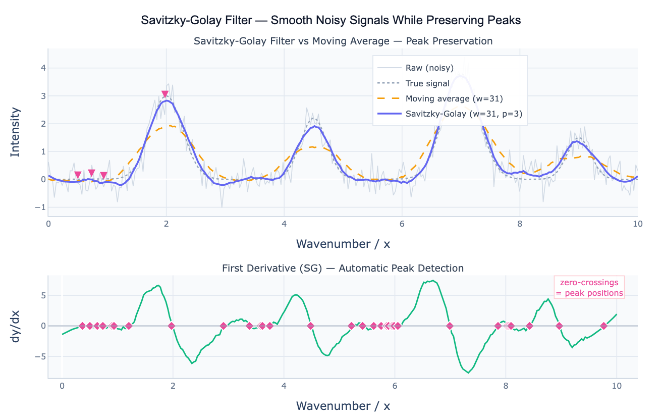
The Savitzky-Golay filter (SG filter) smooths a noisy signal by fitting a local polynomial to each window of w points using least squares, then evaluating the polynomial at the center point. Unlike the simple moving average, which fits a constant (degree 0 polynomial) to each window, the SG filter fits a polynomial of degree p (typically 2–4), which means it can reproduce curved shapes — peaks, valleys, and inflections — within the window without flattening them. The key result: the SG filter preserves the height, width, and position of peaks far better than any equal-width moving average, at the cost of being slightly less aggressive at noise suppression.
This property makes the SG filter the standard smoothing algorithm in spectroscopy: NMR, Raman, IR, UV-Vis, and mass spectrometry all produce signals with sharp peaks whose precise height and position carry chemical information. A moving average would broaden and shrink these peaks; the SG filter tracks their true shape. Beyond spectroscopy, the SG filter is widely used in chromatography (preserving chromatogram peak areas), biomedical signal processing (ECG, EEG), climate science (smoothing temperature records while preserving rapid warming events), and sensor data (accelerometers, pressure gauges) where fast transients matter.
A second critical capability distinguishes the SG filter from all other smoothers: it can directly compute numerical derivatives of a noisy signal. By evaluating the derivative of the fitted local polynomial rather than its value, the filter produces a smoothed first, second, or higher derivative — which would be dominated by noise if computed by finite differences on the raw data. The first derivative is used for peak detection (peaks occur where dy/dx = 0 changes from positive to negative) and for computing rates of change. The second derivative is used for peak sharpening, resolving overlapping peaks, and detecting inflection points in trend data.
How It Works
- Upload your data — provide a CSV or Excel file with an x column (wavenumber, time, distance) and a y column (intensity, value, signal). One row per data point.
- Describe the analysis — e.g. "SG filter window=21 polyorder=3; compare to moving average; compute first derivative; detect peaks from zero-crossings"
- Get full results — the AI writes Python code using scipy.signal.savgol_filter and Plotly to render the smoothed signal, derivative plots, and peak annotations
Required Data Format
| Column | Description | Example |
|---|---|---|
x | Independent variable | 400, 401, 402 (wavenumber cm⁻¹) or 1, 2, 3 (time) |
y | Signal to smooth | 0.23, 1.45, 2.81 (intensity, counts, value) |
Any column names work — describe them in your prompt. Data should be regularly spaced (equal x intervals); if not, ask the AI to resample first.
Interpreting the Results
| Output | What it means |
|---|---|
| SG smoothed signal | Polynomial-fitted smooth — preserves peak heights and positions better than moving average |
| First derivative (dy/dx) | Rate of change — zero-crossings from + to − = signal peaks; from − to + = troughs |
| Second derivative (d²y/dx²) | Curvature — negative at peaks, useful for resolving overlapping bands |
| Window size w | Must be odd; larger = smoother but more peak broadening; typical range 5–51 |
| Polynomial order p | Must be < w; higher order = better peak preservation; typical p = 2 or 3 |
| Comparison to SMA | SG better preserves peak heights; SMA produces lower overall noise — tradeoff |
| Residuals (raw − SG) | Should be random noise; systematic structure = p too low for the signal shape |
Example Prompts
| Scenario | What to type |
|---|---|
| Basic smoothing | SG filter window=21 polyorder=3 on spectral data; overlay on raw; compare to SMA(21) |
| Peak detection | SG smooth then first derivative; find peaks where derivative changes sign from + to −; report peak positions and heights |
| Derivative plot | compute and plot first and second derivatives of the signal using SG window=25 polyorder=4 |
| Window comparison | apply SG with windows 11, 21, and 41 (all polyorder=3); overlay; which window preserves the smallest peaks? |
| Overlapping peaks | second derivative plot to resolve overlapping peaks; annotate each minimum (= peak center in 2nd deriv) |
| Chromatogram | SG filter (window=15, polyorder=2) on chromatogram; detect peaks from first derivative zero-crossings; report retention times and peak areas |
Assumptions to Check
- Regular spacing —
savgol_filterrequires evenly spaced x values; if your data has gaps or irregular spacing, resample to a uniform grid first - Window size odd and > polyorder — the window must be odd (so there is a well-defined center) and strictly greater than the polynomial order: w > p
- Window << signal features — the window should be smaller than the narrowest feature you want to preserve; a window wider than a peak will smooth it away even with high polynomial order
- Polyorder 2 or 3 for most applications — p = 2 or 3 is the standard choice; higher orders (4–5) can overfit to noise at the window edges
- Edge effects — the first and last (w−1)/2 points use reflected or truncated windows (depending on
mode) and may show artifacts; inspect the edges of your filtered output
Related Tools
Use the Moving Average Calculator when you need a simpler, computationally cheaper smoother and peak preservation is not critical. Use the Moving Median Filter when your data contains isolated spike outliers (the SG filter is not robust to outliers — a single spike distorts the local polynomial fit). Use the Gaussian Peak Fit or Lorentzian Peak Fit to fit explicit parametric peak models to the smoothed spectrum after SG filtering. Use the Time Series Decomposition tool for time series with trend and seasonality rather than a spectral signal with peaks.
Frequently Asked Questions
When should I use Savitzky-Golay instead of a moving average? Use the SG filter whenever the shape of features in your signal matters — peak heights, widths, and positions; rates of change (via derivatives); inflection points. The SG filter preserves these at the cost of slightly more residual noise. Use the moving average when you only care about the overall trend and have no narrow peaks to preserve, or when simplicity matters (SMA is trivial to reproduce in any spreadsheet). A practical test: apply both and check whether the peaks in the SG output are taller and narrower than in the SMA output — they should be.
How do I choose window size and polynomial order? The window size w should be approximately 3–5× the FWHM (full width at half maximum) of the narrowest feature you want to smooth without distorting. A window much larger than the feature width will broaden and reduce peak height; a window smaller than the feature width provides little smoothing benefit. Start with w = FWHM × 4 and adjust. The polynomial order p = 2 catches parabolic shapes (most peaks); p = 3 adds an asymmetry term and is the most common choice for spectroscopy; p = 4 or 5 is rarely needed and can overfit noise at the window edges.
Can the SG filter compute numerical derivatives?
Yes — this is one of its major advantages. scipy.signal.savgol_filter(y, window, polyorder, deriv=1) returns the first derivative dy/dx evaluated by differentiating the locally fitted polynomial, which is far less noisy than finite differences on the raw signal. The second derivative (deriv=2) is used in spectroscopy to resolve overlapping peaks: each peak in the original signal appears as a negative minimum in the second derivative, and overlapping peaks that appear as shoulders become distinct minima. Ask the AI to "compute the second derivative with SG window=21 polyorder=4; find minima to resolve overlapping peaks".
My filtered signal has artifacts at the edges — what's wrong?
Edge effects are inherent to any sliding-window filter. At the first and last (w−1)/2 points, there are not enough data points on one side to fill the window, so savgol_filter uses one of several boundary modes (mirror, nearest, wrap, constant). The mirror mode (default) reflects the signal at the boundary — adequate for most cases but can introduce spurious oscillations if the signal changes sharply near the edge. Solutions: (1) trim the first and last (w−1)/2 points from the output before plotting; (2) use mode='nearest' which pads with the endpoint value; (3) extend your data with a few padding points before filtering and remove them afterward.