Time Series Decomposition Tool for Excel & CSV
Decompose time series online from Excel or CSV data. Separate trend, seasonality, and residual structure with AI.
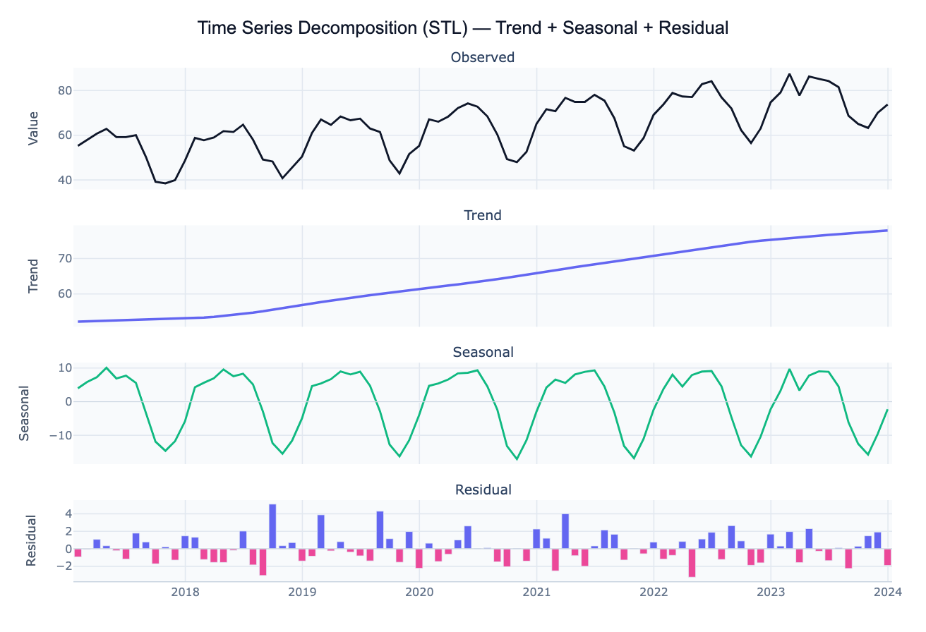
Or try with a sample dataset:
Preview
What Is Time Series Decomposition?
Time series decomposition splits an observed time series into three interpretable components: trend (the long-run direction — increasing, decreasing, or stable), seasonal (a repeating pattern over a fixed period — monthly, quarterly, or weekly cycles), and residual (the remainder after removing trend and seasonality — irregular fluctuations, noise, and one-off events). The decomposition equation is either additive (Observed = Trend + Seasonal + Residual, appropriate when the seasonal amplitude is roughly constant over time) or multiplicative (Observed = Trend × Seasonal × Residual, appropriate when the seasonal amplitude grows with the level of the series).
The most robust modern method is STL (Seasonal and Trend decomposition using LOESS), which uses locally weighted regression (LOESS) to fit both the trend and seasonal components non-parametrically. Unlike classical decomposition (which applies simple moving averages), STL can handle changing seasonal patterns and is robust to outliers. The strength of trend — computed as 1 − Var(Residual)/Var(Trend + Residual) — and the strength of seasonality — 1 − Var(Residual)/Var(Seasonal + Residual) — quantify how much of the total variation each component explains. Values near 1 indicate a strongly structured series; values near 0 indicate a noisy, unstructured one.
How It Works
- Upload your data — provide a CSV or Excel file with a date column (any date format) and a value column (numeric). Data should be regularly spaced — daily, weekly, monthly, quarterly, or annual. One row per time point.
- Describe the analysis — e.g. "STL decomposition with monthly period; plot all four panels; report trend slope and seasonal amplitude; flag residual outliers"
- Get full results — the AI writes Python code using statsmodels STL and Plotly to produce the four-panel decomposition chart plus a component statistics table
Required Data Format
| Column | Description | Example |
|---|---|---|
date | Date or timestamp (any format) | 2020-01, Jan 2020, 2020-01-31 |
value | Numeric time series | 245.3, 312.1, 198.8 (sales, temperature, etc.) |
Any column names work — describe them in your prompt. The series must be regularly spaced (no missing dates); ask the AI to fill gaps with linear interpolation if needed.
Interpreting the Results
| Component | What it means |
|---|---|
| Trend | Smoothed long-run direction — rising, falling, or changing slope |
| Seasonal | Repeating cycle at the specified period — e.g. monthly highs in December |
| Residual | What's left after removing trend and seasonality — noise, outliers, shocks |
| Strength of trend | 1 − Var(R)/Var(T+R) — near 1 = strong trend, near 0 = weak/absent trend |
| Strength of seasonality | 1 − Var(R)/Var(S+R) — near 1 = strong seasonal pattern |
| Residual spike | A large residual at a specific date signals an unusual event — investigation warranted |
| Changing seasonal amplitude | Seasonal component that grows over time → use multiplicative decomposition |
| Trend change point | Sudden shift in the trend component — may indicate a policy change or structural break |
Example Prompts
| Scenario | What to type |
|---|---|
| Basic decomposition | STL decomposition of monthly sales; period 12; 4-panel plot; report trend slope and seasonal amplitude |
| Additive vs multiplicative | compare additive and multiplicative decomposition; which fits better for this series? |
| Outlier detection | STL decomposition; flag residuals more than 2 SD from zero as anomalies; annotate dates on the original series |
| Seasonal strength | decompose weekly website traffic; report strength of trend and seasonality; which day of week is the seasonal peak? |
| Deseasonalized series | STL decomposition; plot original and deseasonalized (trend + residual) on same axes; compute year-over-year growth rate |
| Multiple series | decompose monthly revenue for each product in 'product' column; compare seasonal patterns side by side |
Assumptions to Check
- Regular spacing — STL requires evenly spaced observations; irregular or missing dates must be filled or resampled before decomposition
- Correct period — the seasonal period (12 for monthly, 7 for daily-with-weekly-cycle, 4 for quarterly) must match the actual data frequency; wrong period produces artifacts in the seasonal component
- Additive vs multiplicative — if the peaks and troughs grow proportionally with the trend level, use multiplicative (or log-transform the series and apply additive decomposition)
- Sufficient history — reliable seasonal estimation requires at least 2–3 full seasonal cycles (e.g. at least 2 years of monthly data); STL with fewer cycles produces unstable seasonal estimates
- Stationarity not required — unlike ARIMA, STL decomposition does not require a stationary series; it explicitly extracts the non-stationary trend
Related Tools
Use the Logistic Growth Curve Fit when your time series follows an S-shaped growth curve converging to a plateau rather than showing seasonal cycles. Use the Polynomial Regression tool to fit a smooth trend curve directly to a non-seasonal time series. Use the Correlation Matrix Calculator to explore cross-correlations between multiple time series after decomposition.
Frequently Asked Questions
What is the difference between STL and classical decomposition?Classical decomposition uses centered moving averages to extract the trend, then averages the detrended values by period to get the seasonal component — it's simple but assumes the seasonal pattern is constant over time and is sensitive to outliers. STL uses locally weighted regression (LOESS) for both trend and seasonal, can handle changing seasonal patterns, and has a robust variant that down-weights outliers. STL is generally preferred. Ask the AI to "use STL with robust=True to reduce the influence of outliers on the trend".
How do I choose the right seasonal period? The period equals the number of observations in one full cycle: 12 for monthly data with an annual cycle, 7 for daily data with a weekly cycle, 4 for quarterly data, 52 for weekly data with an annual cycle, 24 for hourly data with a daily cycle. If you're unsure, ask the AI to "plot the autocorrelation function (ACF) to identify the dominant seasonal period before decomposing".
My residuals show a pattern — what does that mean? Structured residuals (systematic waves or trend) mean the decomposition didn't fully capture the signal. Possible reasons: the period is wrong (the seasonality has a different cycle than specified), there is a second seasonality at a different frequency (e.g. weekly + annual), or the series is non-additive (try multiplicative). Ask the AI to "fit STL with multiple seasonal periods using MSTL (multiple seasonal STL)" for data with nested seasonality.
How do I detect anomalies / outliers with decomposition? After STL decomposition, the residual component should be approximately normally distributed with mean zero. Observations where the residual exceeds ±2 or ±3 standard deviations are statistical anomalies — likely real-world events (data errors, policy changes, natural disasters, promotions). Ask the AI to "flag dates where the STL residual exceeds 2.5 standard deviations and annotate them on the original series plot".
Can I use decomposition for forecasting? Yes — a simple forecast projects the extracted trend forward and adds back the seasonal component from the most recent full cycle. For more accurate forecasts, use the decomposed components as inputs to an ARIMA or ETS model (the "Forecast by Decomposition" approach). Ask the AI to "decompose the series and forecast the next 12 months by projecting the trend linearly and repeating the seasonal cycle".