Correlation Matrix Calculator for Excel & CSV
Create correlation matrices online from Excel and CSV data. Measure pairwise relationships and generate correlation heatmaps with AI.
Or try with a sample dataset:
Preview
What Is a Correlation Matrix?
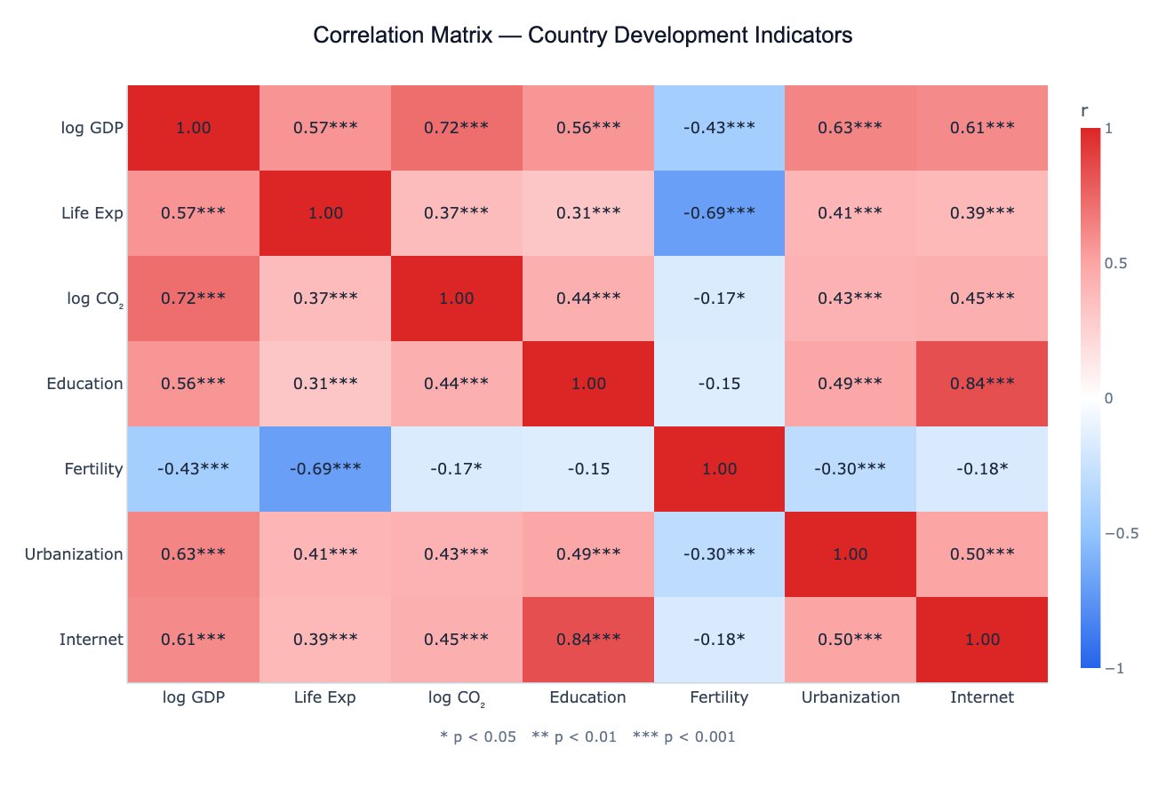
A correlation matrix is a table showing the pairwise correlation coefficients between every combination of numeric variables in a dataset. Each cell contains a value between −1 and +1: +1 means the two variables increase together perfectly, −1 means one increases as the other decreases perfectly, and 0 means no linear relationship. Visualized as a color-coded heatmap with a diverging scale (typically blue for negative, white for zero, red for positive), the correlation matrix lets you scan the strength and direction of all pairwise relationships at a single glance.
The most common measure is the Pearson correlation coefficient (r), which captures linear relationships and assumes the variables are approximately normally distributed. For data with outliers, non-normal distributions, or ordinal scales, Spearman's rank correlation (ρ) is more robust — it ranks the values first and then computes Pearson on the ranks. Each correlation can be accompanied by a p-value indicating whether the observed correlation could plausibly have arisen by chance in a dataset of that size. With 100+ observations, even r = 0.2 can be statistically significant; with 10 observations, r = 0.5 may not be.
Correlation matrices are the standard first diagnostic before any multivariate analysis. In regression, highly correlated predictors (r > 0.8) signal multicollinearity — they carry redundant information and inflate standard errors. In PCA, variable clusters in the correlation matrix predict which groups of variables will collapse into the same principal component. In feature selection for machine learning, pairs with high mutual correlation are candidates for dropping one. In finance, a portfolio's correlation matrix reveals diversification opportunities — pairs of assets with low or negative correlation reduce portfolio volatility.
How It Works
- Upload your data — provide a CSV or Excel file with multiple numeric columns. One row per observation.
- Describe the analysis — e.g. "Pearson correlation matrix of all numeric columns, annotate with r and p-values, cluster by correlation"
- Get full results — the AI writes Python code using pandas and scipy to compute correlations and p-values, and Plotly to render the heatmap with annotations
Interpreting the Results
| Cell value | What it means |
|---|---|
| r = +1.0 | Perfect positive linear relationship |
| r = +0.7 to +0.9 | Strong positive correlation |
| r = +0.3 to +0.6 | Moderate positive correlation |
| r near 0 | Little or no linear relationship |
| r = −0.3 to −0.6 | Moderate negative correlation |
| r = −0.7 to −0.9 | Strong negative correlation |
| r = −1.0 | Perfect negative linear relationship |
| ***** | p < 0.05 — correlation is statistically significant |
| ****** | p < 0.01 |
| ******* | p < 0.001 |
| Cluster of red cells | Group of mutually correlated variables — may be redundant |
| Blue cell between two red clusters | Two variable groups that move in opposite directions |
Example Prompts
| Scenario | What to type |
|---|---|
| Full matrix | correlation matrix of all numeric columns, Pearson r with p-values, red-blue heatmap |
| Spearman | `Spearman correlation matrix of health indicators, cluster variables, highlight |
| Partial correlations | correlation matrix of stock returns, show which assets are most diversified |
| Significance filter | correlation matrix, mask cells where p > 0.05 (show only significant correlations) |
| Time-lagged | correlation matrix with lag 1 to see how this month's variable predicts next month's |
Assumptions to Check
- Numeric variables — Pearson correlation requires numeric data; for ordinal or ranked data use Spearman
- Sufficient sample size — at least 30 observations for reliable correlation estimates; p-values are unreliable with fewer than 20
- No extreme outliers — a single outlier can dramatically change a Pearson correlation; use Spearman if outliers are present
- Linear relationships — Pearson measures only linear association; two variables can have a strong curved relationship yet r ≈ 0
- Multiple testing — computing n×(n−1)/2 correlations inflates false discovery rate; ask for Bonferroni or FDR correction if testing many pairs
Related Tools
Use the Pair Plot Generator to visualize the actual scatter of each variable pair after the correlation matrix identifies which pairs are most interesting. Use the PCA tool after identifying correlated variable clusters — PCA will compress those clusters into fewer components. Use the Exploratory Data Analysis tool for a full automated analysis that includes the correlation matrix, distributions, and outlier summary in one report.
Frequently Asked Questions
What's the difference between Pearson and Spearman correlation?Pearson measures linear association between raw values — it assumes both variables are roughly normally distributed and is sensitive to outliers. Spearman ranks all values first and then computes Pearson on the ranks — it measures monotonic association (variables that consistently increase together, even non-linearly) and is robust to outliers and non-normal distributions. Use Spearman when your data has skew, outliers, or ordinal scales; use Pearson for roughly normal, continuous data without extreme outliers.
My matrix has 40+ variables — can I still use it? A 40×40 matrix has 780 cells and becomes hard to read. Ask the AI to: (1) cluster the heatmap (reorder rows/columns so correlated variables are adjacent), (2) show only the lower triangle, (3) mask non-significant cells (set them to white), or (4) threshold (show only |r| > 0.5). For very many variables, the PCA tool or a network graph of significant correlations may be more useful.
High correlation doesn't mean one variable causes the other — how do I check? Correlation is not causation. A high r between, say, ice cream sales and drowning rates doesn't mean ice cream causes drowning (both are driven by summer heat). To make causal claims you need experimental design or causal inference methods (instrumental variables, difference-in-differences, etc.). The correlation matrix is purely descriptive.
Can I compute partial correlations — controlling for a third variable? Yes — ask for "partial correlation between X and Y controlling for Z". Partial correlation removes the shared influence of control variables and shows the unique linear relationship between two variables. This is especially useful when a confounding variable drives spurious correlations (e.g. GDP driving both CO₂ and life expectancy, making them appear correlated even after controlling for GDP).
What does it mean if my correlation matrix is not positive semi-definite? A valid correlation matrix must be positive semi-definite (all eigenvalues ≥ 0). This can fail when you have missing data handled by pairwise deletion (each pair computed on different samples) or when rounding introduces inconsistencies. Ask the AI to use listwise deletion (same rows for all pairs) or apply nearest positive definite correction to fix it.