Polynomial Regression Calculator for Excel & CSV
Run polynomial regression online from Excel or CSV data. Fit curved relationships, compare degrees, and inspect model fit with AI.
Or try with a sample dataset:
Preview
What Is Polynomial Regression?
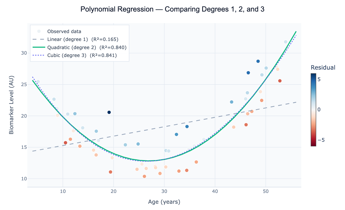
Polynomial regression extends linear regression to model curved relationships between a predictor variable x and an outcome variable y. Instead of fitting a straight line (y = β₀ + β₁x), it fits a polynomial: y = β₀ + β₁x + β₂x² + β₃x³ + … + βₙxⁿ. The degree of the polynomial determines the shape: degree 2 (quadratic) captures U-shaped or inverted-U-shaped curves; degree 3 (cubic) adds an S-shaped inflection; higher degrees fit increasingly complex shapes. Despite using higher powers of x, polynomial regression is still a linear model in the statistical sense — the coefficients β are estimated by ordinary least squares, and all the standard regression diagnostics (R², F-test, confidence intervals) apply directly.
The most common application is fitting data where a straight line clearly misses the curvature. Classic examples include growth curves (plant height vs. days, which accelerates then decelerates), dose-toxicity relationships (low doses are safe, then toxicity rises sharply), environmental Kuznets curves (CO₂ emissions rise with early economic development, then fall as countries grow richer — a quadratic relationship), and age-risk curves (many disease biomarkers follow a U-shaped pattern across the lifespan). Before resorting to complex nonlinear models, a low-degree polynomial often captures the essential shape with interpretable coefficients and well-understood inference procedures.
How It Works
- Upload your data — provide a CSV or Excel file with at least one numeric predictor column and one numeric outcome column. One row per observation.
- Describe the analysis — e.g. "fit polynomial regression of 'temperature' on 'year'; compare degree 1, 2, and 3; report R², AIC, and coefficients; plot fits with 95% confidence bands"
- Get full results — the AI writes Python code using scikit-learn for polynomial feature expansion and scipy.stats for confidence intervals, rendered with Plotly showing overlaid fits and a coefficient table
Required Data Format
| Column | Description | Example |
|---|---|---|
x | Predictor variable (numeric, continuous) | 18, 25, 40, 55 (age in years) |
y | Outcome variable (numeric) | 12.3, 18.7, 31.2 (biomarker level) |
group | Optional: categorical grouping | Male, Female |
Any column names work — describe them in your prompt.
Interpreting the Results
| Output | What it means |
|---|---|
| Degree 1 coefficient (β₁) | Linear slope — rate of change per unit x |
| Degree 2 coefficient (β₂) | Quadratic term — positive = U-shape (minimum), negative = ∩-shape (maximum) |
| Vertex of quadratic | x at maximum/minimum = −β₁/(2β₂) |
| R² | Proportion of variance explained — increases with degree, so compare by AIC not raw R² |
| AIC / BIC | Penalized fit measure — lower is better; use to choose degree without overfitting |
| Confidence band | Range of plausible mean y values at each x — widens toward the edges of the data |
| Prediction interval | Range for a new individual observation — always wider than confidence band |
| Residual plot | Should be random scatter; systematic curvature = the degree is still too low |
Example Prompts
| Scenario | What to type |
|---|---|
| Choose best degree | fit polynomial degrees 1–4 to data; compare R² and AIC; plot best degree with confidence band |
| Quadratic with vertex | quadratic regression of y on x; report vertex (x at minimum/maximum); 95% CI on vertex location |
| Centered polynomial | fit degree-2 polynomial; center x at its mean before squaring to reduce multicollinearity; report coefficients |
| Group comparison | fit quadratic for each group in 'gender' column; overlay on one plot; compare curvature coefficients |
| Extrapolation warning | fit cubic regression; plot fit; shade the extrapolation region outside the training data range |
| Full inference | polynomial regression degree 2; ANOVA table; F-test for the quadratic term; standardized coefficients |
Assumptions to Check
- Representative x range — polynomial fits extrapolate wildly outside the data range; never use a polynomial for prediction beyond the observed x values
- No overfitting — adding more terms always increases R², but high-degree polynomials oscillate between data points (Runge's phenomenon); use AIC/BIC or cross-validation to select degree, not raw R²
- Residual normality and homoscedasticity — the same assumptions as linear regression: residuals should be approximately normal with constant variance across x
- Multicollinearity between powers — x and x² are correlated, which inflates coefficient standard errors; centering x (subtracting the mean) before fitting substantially reduces this
- Sufficient data — a degree-n polynomial has n+1 parameters; you need at least 5–10 observations per coefficient for stable estimation
Related Tools
Use the Linear Regression tool when the relationship is straight (degree 1) — it provides the same output more simply. Use the Multiple Regression tool when you have several predictors; polynomial regression of x is equivalent to multiple regression with x, x², x³ as separate predictors. Use the Residual Plot Generator after fitting to check whether curvature remains in the residuals, which indicates the chosen degree is insufficient.
Frequently Asked Questions
How do I choose the right polynomial degree? The best approach is model comparison by AIC (Akaike Information Criterion) or BIC: fit degrees 1 through (say) 5, compute AIC for each, and choose the degree with the lowest AIC. AIC penalizes extra parameters, preventing overfitting. Alternatively, use cross-validation: split the data into training and test sets, fit each degree on training, evaluate prediction error on test. Never use R² alone — it always increases with degree. Ask the AI to "fit degrees 1–5 and plot AIC vs degree to identify the elbow".
What is the difference between polynomial regression and spline regression? Both model curves, but differently. Polynomial regression uses a single global polynomial across all x values — it can oscillate wildly at the edges. Spline regression (or generalized additive models) joins several lower-degree polynomials at knot points, producing a smooth but locally flexible curve that doesn't oscillate. For datasets with many observations and complex shapes, splines are generally preferred. Ask the AI to fit a cubic spline or use LOWESS smoothing as alternatives to high-degree polynomials.
My quadratic coefficient is not statistically significant — should I drop it? If the F-test for the quadratic term (β₂) is not significant (p > 0.05), the data doesn't support curvature at the current sample size. In that case, drop to degree 1 (linear regression). However, be cautious: insufficient statistical power (small n) can mask real curvature. If the residual plot from a linear fit shows a systematic arch, fit the quadratic regardless of p-value and report both models.
Can I fit a polynomial with multiple predictor variables? Yes — this produces polynomial features in multiple dimensions. For two predictors x₁ and x₂, a degree-2 model includes x₁, x₂, x₁², x₂², and the interaction x₁×x₂. Ask the AI to "fit degree-2 polynomial regression with predictors 'temperature' and 'humidity'; include all interaction and squared terms; report which terms are significant". This quickly becomes parameter-heavy, so ensure sufficient data.
What does the confidence band represent and why does it widen at the edges? The confidence band shows the uncertainty in the mean predicted y at each x value. It is narrowest near the center of the data (where the model is best anchored) and widens at the edges because the polynomial is less constrained there — small changes in coefficients have large effects on the curve away from the centroid. The prediction interval (wider still) adds residual scatter and represents where a new individual observation is expected to fall.