Lorentzian Peak Fit Calculator
Fit Lorentzian peaks online from Excel or CSV data. Estimate center, width, amplitude, and residual diagnostics with AI.
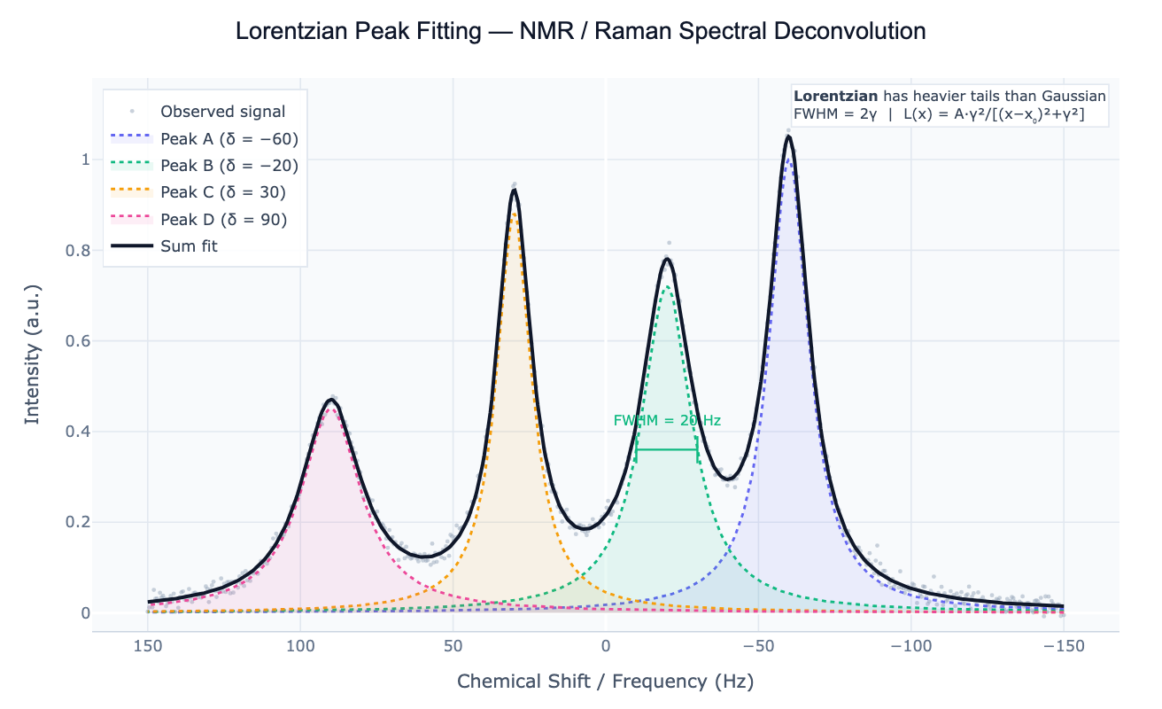
Preview
What Is a Lorentzian Peak?
A Lorentzian (also called a Cauchy distribution in statistics) is a symmetric peak-shaped function defined as L(x) = A × γ² / (x − x₀)² + γ², where A is the peak amplitude, x₀ is the peak center, and γ is the half-width at half maximum (HWHM). The full width at half maximum is FWHM = 2γ. Unlike the Gaussian, which falls off as a squared exponential and has negligible tails beyond a few widths, the Lorentzian falls off as 1/x² and has heavy algebraic tails — a defining feature that makes it physically correct for many spectroscopic systems.
Lorentzian lineshapes arise from homogeneous broadening mechanisms: natural lifetime broadening (governed by the Heisenberg uncertainty principle), collisional broadening in gases, and spin relaxation in NMR. In NMR spectroscopy, every peak in a ¹H, ¹³C, or ³¹P spectrum is a Lorentzian — the linewidth (in Hz) is directly related to the transverse relaxation time T₂ by FWHM = 1/(πT₂). In Raman spectroscopy, phonon modes in crystalline materials produce Lorentzian peaks whose width reports on phonon lifetime and defect density. In resonance physics, the cross-section near a resonance (e.g. optical cavity resonance, atomic absorption line) follows a Lorentzian described by the Breit-Wigner formula. In these contexts, fitting a Gaussian instead of a Lorentzian systematically underestimates the tails and over-estimates narrow linewidths.
How It Works
- Upload your data — provide a CSV or Excel file with an x column (chemical shift in ppm, wavenumber in cm⁻¹, frequency in Hz, or any continuous variable) and a y column (intensity, counts, absorbance). One row per data point.
- Describe the analysis — e.g. "fit 4 Lorentzian peaks to the NMR spectrum; x column is 'ppm', y is 'intensity'; report chemical shifts, FWHM linewidths, and relative integrals; plot individual components and sum"
- Get full results — the AI writes Python code using scipy.optimize.curve_fit to fit the multi-Lorentzian model and Plotly to render the deconvoluted spectrum with filled components, total fit overlay, and parameter table
Required Data Format
| Column | Description | Example |
|---|---|---|
x | Independent variable | 7.25, 7.26, 7.27 … (ppm) |
y | Signal intensity | 0.02, 0.45, 1.00 (a.u.) |
Any column names work — describe them in your prompt. NMR data is typically exported from spectrometer software as a two-column CSV. For Raman or FTIR, export the spectral window of interest.
Interpreting the Results
| Parameter | What it means |
|---|---|
| Peak center x₀ | Position of maximum — chemical shift (ppm), wavenumber (cm⁻¹), frequency (Hz) |
| Amplitude A | Peak height at x₀ |
| γ (HWHM) | Half-width at half maximum — FWHM = 2γ |
| FWHM | Full linewidth — inversely related to T₂ relaxation time in NMR |
| Integrated area = Aπγ | Proportional to the number of nuclei (NMR) or scatterers (Raman) |
| Relative area (%) | Ratio of integrals — corresponds to proton count ratio in ¹H NMR |
| Q-factor = x₀ / FWHM | Resonance quality factor for cavity/resonator measurements |
| Residuals | Flat random scatter = good fit; systematic structure = missing peak or wrong model |
Example Prompts
| Scenario | What to type |
|---|---|
| NMR deconvolution | fit Lorentzian peaks to ¹H NMR; x is 'ppm', y is 'intensity'; report chemical shifts and relative integrals |
| Raman band analysis | fit 3 Lorentzian peaks to Raman spectrum 1200–1700 cm⁻¹; report band positions, FWHM, and areas |
| Linewidth / T₂ | fit Lorentzian to NMR peak; report FWHM in Hz; compute T₂ = 1/(π × FWHM) |
| Overlapping NMR peaks | deconvolute overlapping doublet at 3.5 ppm; fit 2 Lorentzians with equal widths; coupling constant from peak separation |
| Voigt fit comparison | fit Lorentzian, Gaussian, and Voigt to same peak; compare AIC and residuals; report best-fit FWHM |
| Baseline + peaks | fit 4 Lorentzian peaks plus cubic spline baseline to FTIR spectrum; report integrated absorbances |
Assumptions to Check
- Lorentzian is the correct model — Lorentzian is appropriate for homogeneously broadened lines (NMR T₂ relaxation, natural linewidth, phonon lifetime). For inhomogeneously broadened lines (e.g. solid-state NMR powder patterns, optical absorption bands in solution), a Gaussian or Voigt (Lorentzian ⊗ Gaussian) is more appropriate
- Baseline subtracted — Lorentzian tails extend far from the peak center; a sloping or curved baseline significantly distorts the fitted γ and amplitude. Include a polynomial baseline term or pre-process the data
- Good initial guesses — provide approximate peak positions and widths in your prompt: "peaks near 1350 and 1580 cm⁻¹, widths around 20 cm⁻¹". Lorentzian fitting is more sensitive to initial guesses than Gaussian fitting due to the heavy tails
- Avoid fitting noise — very narrow peaks close to the digital resolution of your spectrometer cannot be reliably fit; the Lorentzian γ cannot be smaller than half the point spacing
- Far wings contain information — because Lorentzian tails are heavy, data far from the peak center still influences the fit; ensure the baseline region is correctly modeled
Related Tools
Use the Gaussian Peak Fit when your peaks are inhomogeneously broadened — optical absorption in solution, chromatography peaks, or any system where a distribution of environments broadens the line. Use the Gaussian Peak Fit and ask for a Voigt profile (convolution of Gaussian and Lorentzian) when both broadening mechanisms are present and you want the most accurate lineshape model. Use the Residual Plot Generator to compare fit quality between Lorentzian and Gaussian models systematically.
Frequently Asked Questions
How do I know whether to use Lorentzian or Gaussian for my data? The key diagnostic is the peak tails. Plot your data on a linear scale zoomed out 5–10× the FWHM from the peak center. If the signal decays quickly to baseline (roughly Gaussian), use a Gaussian. If the signal persists far into the wings (slow 1/x² decay), use a Lorentzian. For an objective comparison, fit both models to the same peak, plot the residuals, and compare AIC — the model with lower AIC and flatter residuals is correct. Most NMR peaks are Lorentzian; most optical absorption bands in solution are Gaussian.
What is the Voigt profile and when should I use it? The Voigt profile is the convolution of a Gaussian (width σ) and a Lorentzian (width γ) and represents systems with both homogeneous and inhomogeneous broadening — for example, a gas-phase absorption line that has both Doppler broadening (Gaussian) and collisional broadening (Lorentzian). The Voigt FWHM is approximately 0.5346 × FWHM_L + √(0.2166 × FWHM_L² + FWHM_G²). Ask the AI to "fit a Voigt profile and report the Gaussian and Lorentzian width contributions separately".
My NMR peak has a shoulder — is it one Lorentzian or two? A shoulder usually indicates two overlapping peaks. The reliable test is the second derivative: a single Lorentzian has one minimum in its second derivative; two overlapping peaks produce two minima (often with the shoulder appearing as a slight inflection). Ask the AI to "compute the second derivative of the spectrum to count peaks before fitting". For overlapping NMR doublets, you can also constrain the fit: fix both peaks to have the same width and set their separation equal to the expected J-coupling constant.
How do I extract the spin relaxation time T₂ from a Lorentzian linewidth? In NMR, the transverse relaxation time T₂ is related to the natural linewidth by T₂ = 1/(π × FWHM_Hz), where FWHM must be in Hz (not ppm). Convert ppm to Hz by multiplying by the spectrometer frequency: FWHM_Hz = FWHM_ppm × spectrometer_MHz. Ask the AI to "compute T₂ from the Lorentzian FWHM; spectrometer frequency is 400 MHz; FWHM in ppm".
Can I fit peaks with unequal baselines on the two sides? An asymmetric baseline (one side higher than the other) often indicates either a sloping background or peak overlap with a broad underlying component. The Lorentzian model itself is symmetric. Best practice: (1) fit a local linear baseline using baseline-free spectral windows, (2) subtract it, then (3) fit Lorentzians to the baseline-corrected data. Alternatively, include a linear baseline as two additional free parameters in the fit and let the optimizer determine both baseline and peak parameters simultaneously.