Gaussian Peak Fit Calculator
Fit Gaussian peaks online from Excel or CSV data. Estimate peak center, width, area, and fit quality with AI.
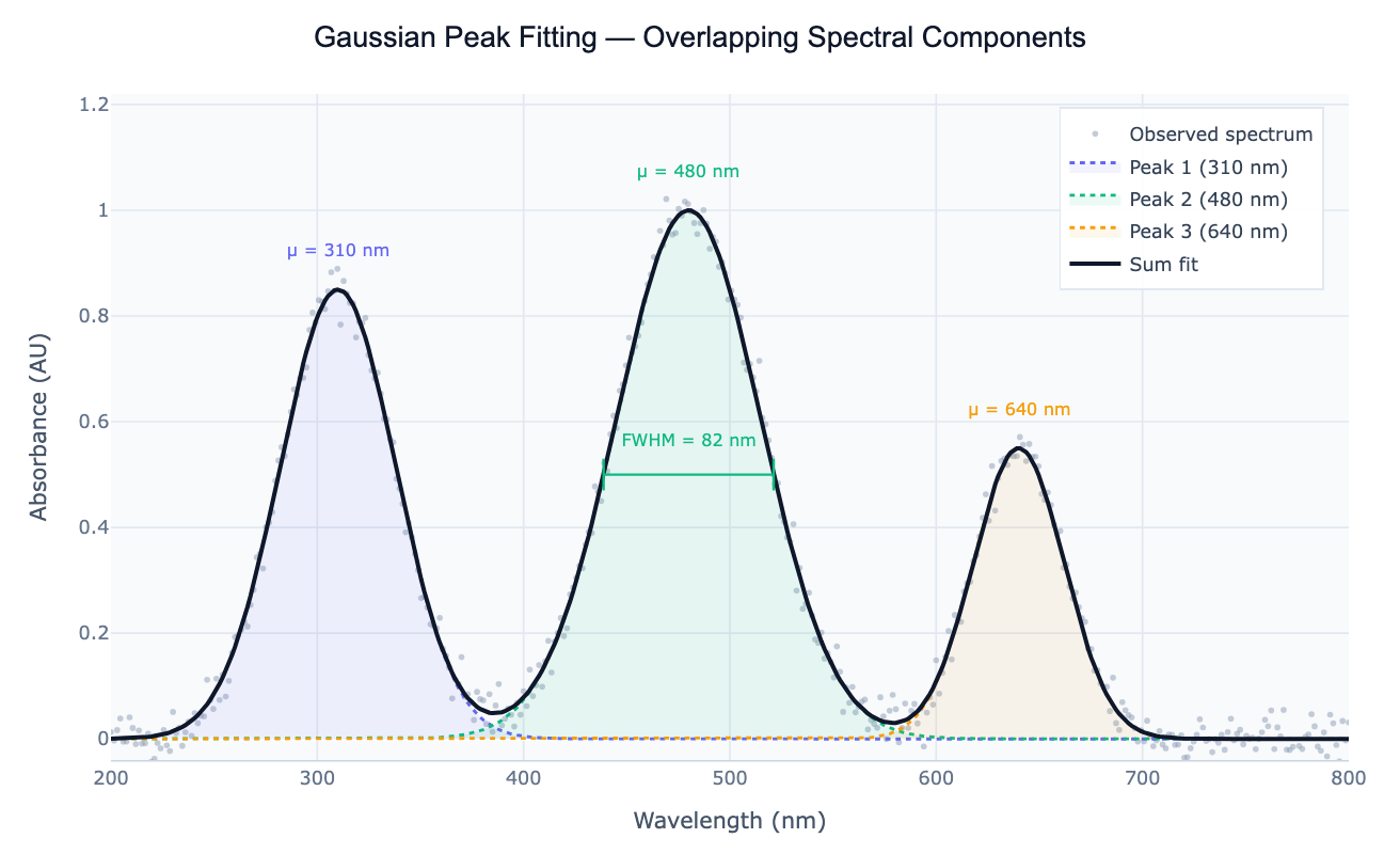
Preview
What Is Gaussian Peak Fitting?
Gaussian peak fitting is the process of modeling a measured signal as the sum of one or more bell-shaped (Gaussian) curves and extracting the parameters of each component: peak center (μ), amplitude (A), and width (σ). A Gaussian peak has the form y = A × exp(−(x − μ)² / (2σ²)), and its full width at half maximum (FWHM = 2.355 × σ) is the most commonly reported width measure. When multiple peaks overlap — as is typical in UV-Vis absorption spectra, fluorescence emission spectra, NMR peaks, chromatography traces, and mass spectra — the individual contributions cannot be read directly from the raw data; nonlinear least-squares fitting deconvolutes them into separate components.
The output of Gaussian peak fitting answers the key questions in spectroscopy and signal analysis: at what wavelength, wavenumber, retention time, or m/z does each component occur? How wide is each peak (resolution)? What is the relative area (proportional to concentration or abundance)? In UV-Vis spectroscopy, overlapping absorption bands from two chromophores can be separated to quantify each species. In fluorescence spectroscopy, a broad emission band may contain contributions from two excited states. In HPLC chromatography, co-eluting compounds produce merged peaks whose individual areas — and therefore concentrations — require peak deconvolution to determine. In Raman and FTIR spectroscopy, Gaussian (or Lorentzian/Voigt) fitting extracts band positions and widths that are sensitive to molecular environment.
How It Works
- Upload your data — provide a CSV or Excel file with an x column (wavelength, wavenumber, retention time, m/z, or any continuous variable) and a y column (absorbance, intensity, counts, signal). One row per data point.
- Describe the analysis — e.g. "fit 3 Gaussian peaks to the absorption spectrum; x column is 'wavelength_nm', y is 'absorbance'; report peak centers, FWHM, and relative areas; plot individual components and sum"
- Get full results — the AI writes Python code using scipy.optimize.curve_fit to fit the multi-Gaussian model and Plotly to render the deconvoluted spectrum with individual peak fills, sum overlay, and parameter table
Required Data Format
| Column | Description | Example |
|---|---|---|
x | Independent variable (continuous) | 300, 301, 302 … (nm) |
y | Signal / response | 0.12, 0.45, 0.89 (absorbance) |
Any column names work — describe them in your prompt. The data should be a densely sampled curve (not raw scatter); typical spectral datasets have 100–1000 points.
Interpreting the Results
| Parameter | What it means |
|---|---|
| Peak center μ | Position of the peak maximum — wavelength, wavenumber, retention time, etc. |
| Amplitude A | Height of the Gaussian at the center |
| σ (sigma) | Standard deviation of the Gaussian — controls width |
| FWHM = 2.355σ | Full width at half maximum — the standard spectral linewidth measure |
| Peak area = A × σ × √(2π) | Proportional to concentration or abundance for quantitative work |
| Relative area (%) | Each peak's area as a fraction of the total fitted area |
| Residuals | Difference between data and sum fit — systematic residuals suggest a missing peak or wrong model |
| R² | Goodness of fit — values > 0.999 are typical for clean spectra |
Example Prompts
| Scenario | What to type |
|---|---|
| Basic deconvolution | fit 3 Gaussian peaks to absorption spectrum; x is 'wavelength_nm', y is 'absorbance'; report μ, FWHM, area for each peak |
| Automatic peak count | determine number of peaks automatically using second derivative; fit Gaussians; report all peak parameters |
| Chromatogram | deconvolute chromatogram peak at 8–12 min into overlapping Gaussians; report retention time, area, and resolution |
| Fluorescence emission | fit 2-component Gaussian to fluorescence emission; fixed baseline at 0; relative areas for quantification |
| With baseline | fit 3 Gaussians plus linear baseline to Raman spectrum; report band positions and integrated intensities |
| Voigt profile | fit Voigt profiles (convolution of Gaussian and Lorentzian) to NMR peaks; compare peak widths |
Assumptions to Check
- Gaussian peak shape — many spectral peaks are better described by Lorentzian (sharp center, wide tails) or Voigt (convolution of Gaussian and Lorentzian) profiles; ask the AI to compare models if residuals show systematic patterns at the peak tails
- Correct number of peaks — Gaussian fitting requires specifying (or estimating) the number of components; use the second derivative of the spectrum to identify inflection points as initial peak position estimates
- Good initial guesses — nonlinear fitting can converge to local minima; provide approximate peak positions and amplitudes in your prompt: "peaks near 310, 480, and 640 nm with amplitudes around 0.9, 1.0, and 0.6"
- Flat or subtracted baseline — a sloping or curved baseline shifts peak positions and widths; fit a polynomial or spline baseline first, or include a baseline term in the model
- No noise preprocessing needed — the fit naturally averages over noise, but very noisy data (SNR < 10) may require light smoothing first
Related Tools
Use the Density Plot Generator to visualize the distribution of a dataset as a smooth curve without fitting a specific peak model. Use the Hill Equation Fit when your peak-like curve follows a sigmoidal saturation model rather than a symmetric Gaussian. Use the Residual Plot Generator to assess fit quality by examining the difference between your data and the fitted model systematically.
Frequently Asked Questions
How do I know how many Gaussian peaks to fit? The most reliable method is the second derivative of the spectrum: negative minima in the second derivative correspond to peak positions. Ask the AI to "find peaks using the second derivative and use those positions as initial guesses for Gaussian fitting". Alternatively, fit increasing numbers of peaks (1, 2, 3…) and compare using AIC (Akaike Information Criterion) — the optimal number minimizes AIC. Visual inspection of residuals also helps: systematic S-shaped residuals indicate a missing component.
What is the difference between Gaussian and Lorentzian peak shapes? A Gaussian has the form exp(−x²/2σ²) and falls off rapidly in the tails — it arises from inhomogeneous broadening (e.g. distributions of molecular environments). A Lorentzian has the form 1/(1 + x²/γ²) and has much heavier tails — it arises from homogeneous broadening (e.g. lifetime broadening). A Voigt profile is the convolution of the two and is most accurate for many spectroscopic lines. Ask the AI to "fit Voigt profiles instead of Gaussians" if your peaks have visible tails.
Can I fit peaks with a sloping or curved background? Yes — include a baseline model in the fit. Common options are a linear baseline (two extra parameters: slope and intercept), polynomial baseline (e.g. quadratic), or a spline baseline estimated from regions with no peaks. Specify in your prompt: "fit 2 Gaussians plus a linear baseline; baseline-free regions are 200–250 nm and 700–750 nm".
How do I use peak areas for quantification? The integrated area of a Gaussian peak is A × σ × √(2π) — directly proportional to the amount of the species if Beer-Lambert linearity holds. For quantitative work, build a calibration curve with known concentrations, extract areas at each concentration, and use linear regression to convert area to concentration. Ask the AI to "compute integrated areas for each peak and normalize to the internal standard peak at 400 nm".
My peaks are very close together — can Gaussian fitting still separate them? Gaussian fitting can resolve peaks that overlap significantly, but the solution becomes non-unique when peaks are closer than about half their FWHM. In that regime, small changes in initial guesses produce different-looking (but statistically equivalent) solutions. Constrain the fit where possible — for example, fix one peak position to a known reference wavelength, or fix the ratio of two peaks based on stoichiometry. Report confidence intervals on peak parameters to communicate the uncertainty.