Moving Average Calculator for Excel & CSV
Calculate moving averages online from Excel or CSV data. Smooth noisy series and compare short-term versus long-term trends with AI.
Or try with a sample dataset:
Preview
What Is a Moving Average?
A moving average smooths a time series by replacing each observation with the average of the surrounding window of w observations, reducing short-term noise and making the underlying trend more visible. The most common type is the simple moving average (SMA): the mean of the w most recent observations, all weighted equally. The exponential moving average (EMA) applies geometrically decreasing weights to older observations, giving more influence to recent values — it reacts faster to new trends than the SMA of the same nominal window. The weighted moving average (WMA) applies explicit custom weights (typically linearly decreasing) that the user specifies. Each type makes a different tradeoff between lag (how quickly the average tracks the true signal) and smoothness (how much short-term noise is suppressed).
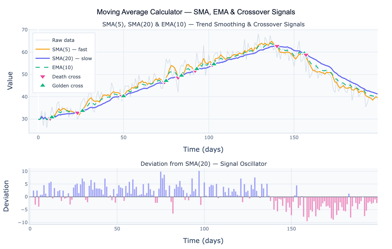
Moving averages are the foundation of a wide range of analytical workflows. In trend analysis, a long-window SMA (e.g. 200-day) defines the primary direction of a time series — values consistently above the SMA indicate an uptrend; below indicates a downtrend. In crossover analysis, two moving averages of different window lengths signal trend reversals: when a fast SMA crosses above a slow SMA (a golden cross), the short-term momentum is accelerating relative to the long-term trend; when the fast crosses below (a death cross), momentum is decelerating. In deseasonalization, a 12-month SMA applied to monthly data exactly removes annual seasonality, leaving a cleaner trend signal. In epidemiology, 7-day moving averages smooth out day-of-week reporting patterns in daily case counts.
The window size is the critical parameter: a small window (e.g. SMA-5) tracks the data closely but retains much noise; a large window (e.g. SMA-50) is smooth but lags behind genuine trend changes by roughly w/2 periods. The deviation oscillator — the difference between the raw series and its moving average — separates the trend from the short-term fluctuations, showing how far above or below the average the current value is. Values consistently above the moving average indicate a bullish or above-trend environment; values persistently below indicate weakness.
How It Works
- Upload your data — provide a CSV or Excel file with a date column and a value column. Daily, weekly, monthly, or annual data all work. One row per time point.
- Describe the analysis — e.g. "SMA(7) and EMA(14) overlaid on daily sales; golden cross / death cross annotations; deviation oscillator below"
- Get full results — the AI writes Python code using pandas rolling/ewm and Plotly to render the multi-MA overlay chart, crossover signal markers, and the deviation oscillator panel
Required Data Format
| Column | Description | Example |
|---|---|---|
date | Date or time index | 2020-01-01, 2020-01, Jan 2020 |
value | Numeric time series | 245.3, 312.1, 198.8 |
Any column names work — describe them in your prompt. For financial OHLC data, specify which column to smooth (close price, volume, etc.).
Interpreting the Results
| Output | What it means |
|---|---|
| SMA(w) | Mean of the w most recent observations — equal weight to all; lags by w/2 periods |
| EMA(span) | Exponentially weighted mean — recent observations weighted more; lower lag than SMA |
| WMA(w) | Linearly weighted mean — most recent observation gets weight w, second most recent w−1, etc. |
| Golden cross | Fast MA crosses above slow MA — short-term momentum accelerating upward |
| Death cross | Fast MA crosses below slow MA — short-term momentum decelerating |
| Deviation oscillator | Raw − SMA — positive = above trend, negative = below trend |
| Lag | The moving average trails real changes by approximately (w−1)/2 periods |
| Window size tradeoff | Larger w = smoother but more lag; smaller w = reactive but noisy |
Example Prompts
| Scenario | What to type |
|---|---|
| Basic smoothing | SMA(7) and SMA(30) overlaid on daily data; which window best shows the underlying trend? |
| EMA vs SMA comparison | compare SMA(20) and EMA(20) on the same chart; annotate where EMA reacts faster to the trend reversal |
| Crossover signals | SMA(5) and SMA(20) crossover signals; annotate golden and death crosses; table of crossover dates |
| Deseasonalization | 12-month SMA to remove annual seasonality from monthly data; plot deseasonalized series |
| Multiple windows | SMA(3), SMA(7), SMA(14), SMA(30) overlaid; which window loses the least detail while still smoothing? |
| Deviation analysis | SMA(20); plot deviation oscillator (raw − SMA); flag months where deviation > 2 standard deviations |
Assumptions to Check
- Regular spacing — moving averages assume evenly spaced observations; irregular timestamps produce distorted windows; resample to a regular frequency first
- Window must be shorter than the series — the window w must be much smaller than the series length n; a window larger than n/3 produces meaningless averages over too few points
- Centered vs trailing window — trailing windows (all w points in the past) have a lag of (w−1)/2; centered windows have no lag but require future data and cannot be used in real-time
- Trend vs seasonal periods — a 12-month SMA applied to monthly data acts as a deseasonalizer; do not use this to estimate the underlying trend if your intent is to preserve seasonal information
- EMA initialization — the first EMA value depends on the initialization method (first-observation start vs warm-up period); ask the AI to use
adjust=Falsefor standard exponential smoothing behavior
Related Tools
Use the Moving Median Filter when your data contains isolated spike outliers that would distort the mean — the median is more robust to extreme values. Use the Time Series Decomposition tool when you want to formally separate trend, seasonal, and residual components rather than just smoothing. Use the Trendline Calculator to fit a parametric (linear or exponential) trend curve rather than a nonparametric moving average. Use the Seasonality Analysis tool to analyze the seasonal pattern that a 12-month moving average removes.
Frequently Asked Questions
What is the difference between SMA, EMA, and WMA?SMA (simple moving average) gives equal weight to all w observations in the window — it is straightforward but lags true changes by (w−1)/2 periods. EMA (exponential moving average) uses geometrically decaying weights so recent observations matter more; for a given nominal window size, the EMA reacts roughly twice as fast as the SMA to new data. WMA (weighted moving average) applies explicit linear weights (most recent = w, previous = w−1, …, oldest = 1) — a middle ground between SMA and EMA. In practice, SMA is the standard for trend identification and deseasonalization; EMA is preferred when faster reaction to recent data is important; WMA is less common but useful when you want a specific weight decay profile.
How do I choose the right window size? The window size should match the timescale of the noise you want to remove. For daily data with a weekly reporting cycle, a 7-day window removes day-of-week effects. For monthly data with an annual seasonal pattern, a 12-month window deseasonalizes. For identifying long-run trends, use a window equal to roughly one-third to one-half of the data span. A practical approach: plot the series with several window sizes (5, 10, 20, 50) and choose the smallest window that produces a visually smooth trend — the smallest window minimizes lag while achieving your smoothing goal.
What is a golden cross and should I trust it as a trading signal? A golden cross occurs when a short-window moving average (e.g. SMA-50) crosses above a long-window moving average (e.g. SMA-200), signaling that recent momentum is stronger than the long-run average. A death cross is the reverse. These are widely followed technical indicators in financial markets, but they are lagging signals — they confirm a trend that has already started rather than predicting it, and they generate many false signals in sideways markets. For scientific and business data, crossover signals are most useful as a simple visual marker for regime changes, not as predictive indicators. Always validate against domain knowledge.
Why does my moving average look flat or have a gap at the start?
Flat values at the start occur when the rolling window uses min_periods=w (requires a full window before computing) — the first w−1 positions are NaN. Set min_periods=1 to start computing from the first observation using partial windows, or accept the NaN gap. The partial-window averages at the start have lower effective sample sizes and are less reliable — plot them in a lighter color or omit them from analysis. For EMA, no gap occurs because the calculation is recursive from the first point.