Meta-Analysis Calculator
Run fixed-effect and random-effects meta-analysis online from Excel or CSV study data. Pool effect sizes, compute I-squared, and generate forest plots with AI.
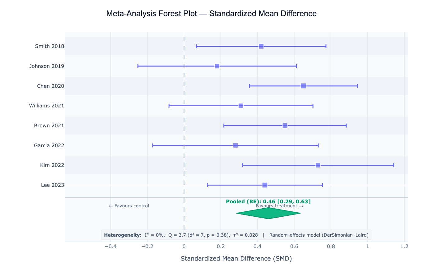
Preview
What Is Meta-Analysis?
Meta-analysis is a statistical technique that combines the results of multiple independent studies addressing the same research question to produce a single, more precise overall estimate of the effect. Individual studies are often underpowered to detect small but clinically meaningful effects; meta-analysis synthesizes their evidence into a pooled estimate with narrower confidence intervals. The central output is a forest plot — a graphical display showing each study's effect estimate with its confidence interval as a horizontal line, with the box size proportional to the study's weight, and a diamond at the bottom representing the pooled estimate. Meta-analysis is the highest level of evidence in evidence-based medicine and is the foundation of systematic reviews, clinical guideline development, and regulatory submissions.
The two fundamental models are fixed-effect and random-effects. The fixed-effect model (Mantel-Haenszel, inverse-variance) assumes all studies estimate the same true effect and that observed differences between studies are due to sampling error alone — appropriate when studies are homogeneous in design, population, and intervention. The random-effects model (DerSimonian-Laird, REML) assumes that the true effect varies across studies due to real between-study differences (different populations, dosages, follow-up times), and estimates both the mean effect and the variance of the true effect distribution (τ²). In practice, random-effects models are preferred when there is any clinical or methodological heterogeneity between studies.
Heterogeneity is the degree to which studies differ in their true effects beyond what sampling error predicts. The I² statistic quantifies the proportion of total variation that is due to between-study variance rather than chance: I² = 0% means all variation is sampling error (homogeneous studies); I² = 25%, 50%, 75% are conventional thresholds for low, moderate, and high heterogeneity. The Cochran's Q test tests whether heterogeneity is statistically significant (but has low power with few studies). High I² (> 50%) signals that a single pooled estimate may oversimplify the evidence — subgroup analysis or meta-regression is needed to explain the heterogeneity.
How It Works
- Upload your data — provide a CSV or Excel file with one row per study and columns for study label, effect size, and standard error (or sample sizes and raw counts from which the AI computes effect sizes). Common formats: pre-calculated SMD/OR/RR with SE, or 2×2 tables (events and totals for treatment and control).
- Describe the analysis — e.g. "random-effects meta-analysis of SMD; DerSimonian-Laird estimator; forest plot sorted by effect size; funnel plot; Egger's test for publication bias"
- Get full results — the AI writes Python code using PyMARE or manual numpy/scipy implementations with Plotly to pool effect sizes, compute heterogeneity statistics, generate the forest plot with proportional weight boxes, and produce a funnel plot for bias assessment
Required Data Format
Pre-calculated effects (simplest)
| Column | Description | Example |
|---|---|---|
study | Study label | Smith 2020, RCT-AU-2021 |
effect_size | Effect estimate | 0.42 (SMD), 0.78 (OR), −15.2 (MD) |
se | Standard error of the effect | 0.18 |
n | Optional: total sample size | 120 |
Raw 2×2 table (binary outcomes)
| Column | Description | Example |
|---|---|---|
study | Study label | Jones 2019 |
events_t | Events in treatment group | 23 |
n_t | Total in treatment group | 95 |
events_c | Events in control group | 31 |
n_c | Total in control group | 98 |
Any column names work — describe them in your prompt. The AI will compute the log-OR, log-RR, or risk difference from the raw counts.
Interpreting the Results
| Output | What it means |
|---|---|
| Pooled effect size | Weighted average of study effects — the primary meta-analytic estimate |
| 95% CI on pooled estimate | Uncertainty around the pooled effect; if it excludes the null, the pooled effect is statistically significant |
| I² | % of variance due to between-study heterogeneity — 0%=none, 25%=low, 50%=moderate, 75%=high |
| Cochran's Q | Test of heterogeneity; small p-value = significant heterogeneity (but low power with few studies) |
| τ² (tau²) | Between-study variance in random-effects model — the spread of true effects across studies |
| τ (tau) | SD of true effects — reported in the same units as the effect size; useful for interpreting τ² |
| Study weight | Contribution of each study to the pooled estimate — larger studies and more precise estimates get more weight |
| Forest plot | Per-study CI bars (box size = weight) + pooled diamond; studies whose CI excludes null shown in highlighted color |
| Funnel plot | SE vs effect size; asymmetry suggests publication bias or small-study effects |
| Egger's test | Regression test of funnel plot asymmetry — significant p-value suggests possible publication bias |
| Prediction interval | Range where 95% of future true effects are expected to fall (random-effects only) — wider than CI |
Example Prompts
| Scenario | What to type |
|---|---|
| Basic pooling | random-effects meta-analysis of SMD; DerSimonian-Laird; forest plot; report I², Q, τ² |
| Binary outcomes | pool odds ratios from 2×2 tables; fixed and random effects; compare; log scale forest plot |
| Subgroup analysis | random-effects meta-analysis; subgroup by study design (RCT vs observational); forest plot with subgroup diamonds |
| Publication bias | funnel plot of SE vs effect size; Egger's test; trim-and-fill correction for publication bias |
| Meta-regression | meta-regression with year of publication and sample size as moderators; plot effect size vs year |
| Sensitivity analysis | leave-one-out sensitivity analysis; re-run pooled estimate excluding each study one at a time; plot |
| Prediction interval | random-effects pooling; compute 95% prediction interval; annotate on forest plot alongside CI |
| REML estimator | random-effects meta-analysis with REML estimator for τ²; compare to DL estimator; report both τ² values |
Assumptions to Check
- Comparable effect measure — all studies must report the same effect measure (all SMD, all OR, all RR); mixing effect types is not valid without transformation
- Independent studies — each study must provide an independent data point; pooling multiple arms from the same trial, or multiple studies from the same research group sharing subjects, introduces non-independence
- Studies estimating the same quantity — the PICO framework (Population, Intervention, Comparator, Outcome) must be sufficiently similar across studies; pooling apples and oranges inflates heterogeneity meaninglessly
- Log-scale for ratio measures — odds ratios, risk ratios, and hazard ratios must be log-transformed before pooling (the forest plot x-axis should use log scale); pooling raw ORs is incorrect
- Minimum number of studies — fixed-effect pooling is valid with ≥ 2 studies, but random-effects estimation of τ² is unreliable with fewer than 5–10 studies; with few studies, use a Bayesian approach or report only the fixed-effect estimate
- Publication bias awareness — funnel plot asymmetry and Egger's test are heuristics, not definitive; small-study effects (genuine associations between study size and effect due to clinical reasons) can mimic publication bias
Related Tools
Use the Survival Curve Generator and Cox Proportional Hazards Model to generate study-level hazard ratios that you then pool in a meta-analysis. Use the Forest Plot Generator within this tool — the forest plot is built-in. Use the Chi-Square Test Calculator to analyze individual 2×2 tables before pooling. Use the Correlation Matrix Calculator to explore associations among study-level moderators before running meta-regression.
Frequently Asked Questions
When should I use fixed-effect vs random-effects meta-analysis? Use the fixed-effect model when all studies were conducted under essentially identical conditions (same protocol, population, intervention dose) and you believe there is one true effect that all studies are estimating — typically pre-specified in a protocol or when analyzing tightly controlled laboratory replication studies. Use the random-effects model (almost always in practice) when studies differ in any clinically meaningful way — different populations, dosages, follow-up times, or outcome definitions — because these differences introduce real variability in the true effect. The random-effects model accounts for this between-study variance (τ²) and produces wider, more honest confidence intervals. Choosing fixed-effect because it gives a more significant result is not valid.
What does a prediction interval mean and why is it wider than the confidence interval? The 95% confidence interval (CI) on the pooled estimate describes uncertainty about the mean true effect across studies — it shrinks as you add more studies. The 95% prediction interval (PI) describes where 95% of future individual study true effects are expected to fall, accounting for the between-study variance τ². The PI is always wider than the CI when τ² > 0. Example: if the pooled OR = 0.75 95% CI 0.65–0.87 but the 95% PI = 0.45–1.25, the treatment is beneficial on average but might be ineffective (OR > 1 possible) in some subpopulations. Reporting only the CI without the PI overstates the consistency of evidence when I² is high.
How do I interpret I² and when is heterogeneity a problem? I² = 0–25%: low heterogeneity — studies are fairly consistent and pooling is straightforward. I² = 25–50%: moderate heterogeneity — worth investigating potential moderators but pooling is still reasonable. I² = 50–75%: high heterogeneity — a single pooled estimate may be misleading; explore subgroup analysis or meta-regression to find sources. I² > 75%: very high heterogeneity — question whether pooling is appropriate at all; may need to report studies narratively. Note that I² depends on sample size (more studies → more power to detect heterogeneity) — report τ² alongside I² to describe the magnitude of between-study variation in effect size units.
What is publication bias and how do I detect it?Publication bias occurs because studies with statistically significant or large effects are more likely to be published than null results, making the published literature systematically biased toward larger effects. In a funnel plot (effect size vs standard error), the studies should form a symmetric inverted funnel if there is no bias. Asymmetry — typically an absence of small studies on the left side of the null — suggests that small null or negative studies were never published. Egger's test formally tests for this asymmetry. The trim-and-fill method imputes missing studies to symmetrize the funnel and re-estimates the pooled effect after correction. However, funnel asymmetry can also result from genuine small-study effects (different populations or doses in smaller studies) rather than publication bias — the interpretation always requires clinical judgment.
Can I meta-analyze studies that reported different effect measures? No — you cannot directly pool, for example, odds ratios from some studies and risk differences from others. However, you can convert between measures if you have the raw data: risk difference and relative risk can be derived from each other given the baseline risk; OR can be approximately converted to RR using the formula RR ≈ OR / (1 − p₀ + p₀ × OR) where p₀ is the control group event rate. Alternatively, use the standardized mean difference (SMD) for continuous outcomes where studies used different measurement scales — the SMD divides the mean difference by the pooled SD, making all studies dimensionless and directly comparable.