Sales Forecasting Tool for Excel & CSV
Forecast sales online from Excel or CSV data. Fit ETS and trend models, decompose seasonality, and generate prediction intervals with AI.
Or try with a sample dataset:
Preview
What Is Sales Forecasting?
Sales forecasting is the process of using historical revenue or demand data to project future performance over a specified horizon. Unlike a simple trendline extrapolation, a proper statistical forecast accounts for three components that drive most sales time series: the trend (sustained upward or downward movement over time), seasonality (regular periodic patterns — Q4 spikes, summer dips, monthly cycles), and residual noise (random fluctuations that cannot be predicted). Separating these components and modeling them explicitly produces more accurate and credible forecasts than applying a linear regression to raw monthly totals.
The two most widely used statistical forecasting families are Exponential Smoothing (ETS) and ARIMA. ETS models (Holt-Winters) assign exponentially decreasing weights to older observations, with separate smoothing parameters for level, trend, and seasonality. ETS(A,A,A) — additive error, additive trend, additive seasonality — is appropriate for sales data where seasonal variation is roughly constant in absolute dollars. ETS(A,A,M) — multiplicative seasonality — fits data where the seasonal swing grows proportionally with the overall level (common in fast-growing businesses). ARIMA models capture autocorrelation structure in the residuals after differencing to achieve stationarity; they are particularly useful when seasonality is irregular or when external regressors (promotions, price changes) are included via ARIMAX.
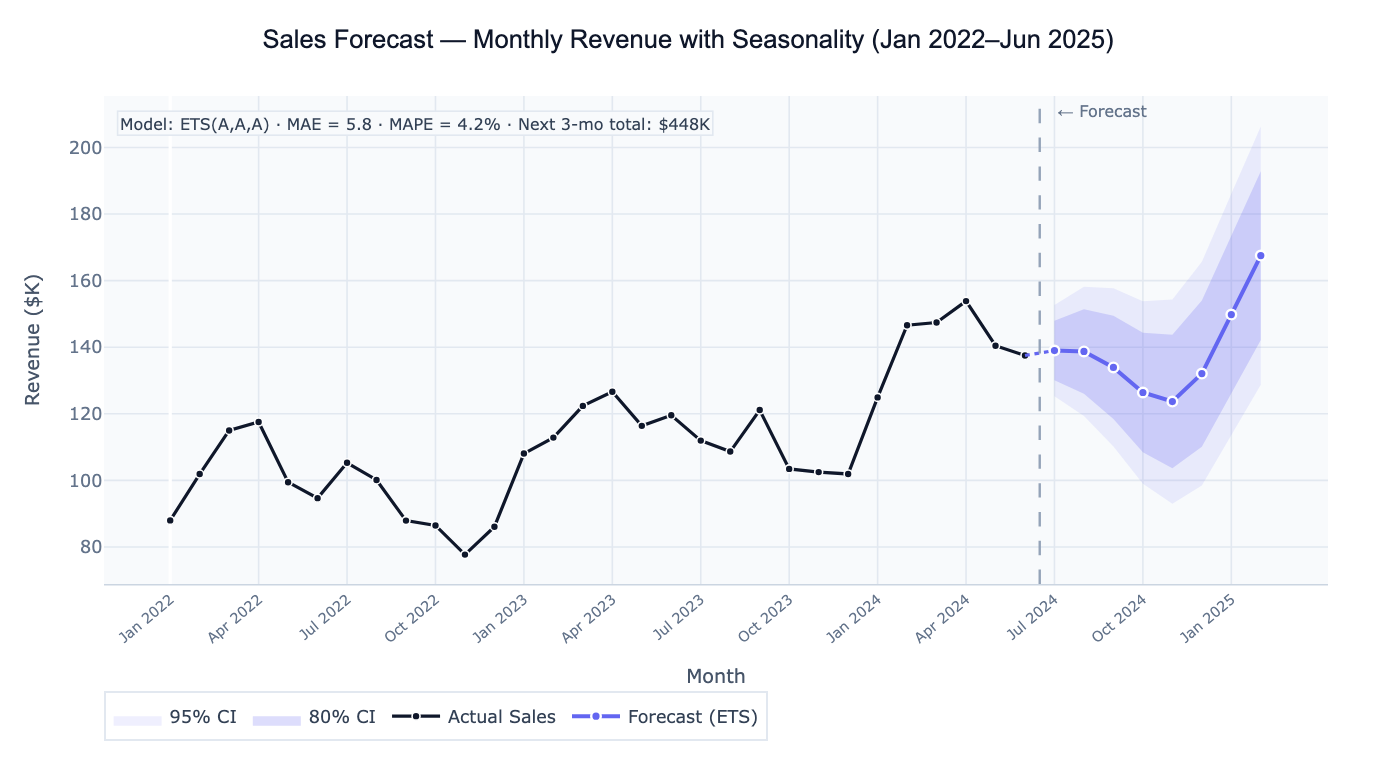
A concrete example: a SaaS company has 30 months of monthly revenue data. ETS(A,A,A) decomposes the series into a +148K to 155K, $182K] by month 6. The expanding uncertainty bands reflect that forecast uncertainty increases with the horizon — the model is confident about next month but less so about 6 months out.
How It Works
- Upload your data — provide a CSV or Excel file with a date/period column and a numeric sales or revenue column. Data should be at consistent intervals (daily, weekly, monthly, quarterly).
- Describe the forecast — e.g. "monthly sales column; forecast next 6 months; ETS with additive seasonality; 80% and 95% prediction intervals; decompose trend and seasonal components; compute MAPE"
- Get full results — the AI writes Python code using statsmodels and Plotly to fit the model, generate forecasts with confidence bands, decompose components, and compute accuracy metrics
Required Data Format
| Column | Description | Example |
|---|---|---|
date | Period identifier | 2024-01, Jan 2024, 2024-01-01 |
sales | Numeric outcome to forecast | 142500, 1284, 98.3 |
segment | Optional: grouping variable | region, product_line |
Any column names work — describe them in your prompt. Data must be at regular intervals. Gaps (missing periods) should be filled with 0 or interpolated — describe your preference. Minimum recommended series length: 2 full seasonal cycles (e.g., 24 months for monthly data with annual seasonality).
Interpreting the Results
| Output | What it means |
|---|---|
| Forecast line | Point estimate of future values — the model's best prediction |
| 80% prediction interval | Range that should contain the true future value 80% of the time |
| 95% prediction interval | Wider range for 95% coverage — use when the cost of being wrong is high |
| MAE | Mean Absolute Error — average forecast error in the original units (e.g., dollars) |
| MAPE | Mean Absolute Percentage Error — average % error; < 10% is good for monthly sales |
| RMSE | Root Mean Squared Error — penalizes large errors more than MAE |
| Trend component | Long-run direction after removing seasonality and noise |
| Seasonal component | Recurring pattern by period (month, quarter) — shows which periods are high/low |
| Residuals | Unexplained variation — should be random (no autocorrelation) for a well-fit model |
Example Prompts
| Scenario | What to type |
|---|---|
| Basic ETS forecast | monthly sales; forecast 6 months; ETS model; 80% and 95% CI; plot with confidence bands |
| Model comparison | compare ETS, ARIMA, and linear trend; select best by AIC; forecast 12 months; accuracy table |
| Seasonal decomposition | decompose into trend, seasonal, and residual components; additive model; plot each component |
| Accuracy on holdout | use last 6 months as test set; fit model on training data; compute MAE and MAPE on holdout |
| Multiple series | forecast sales for each of 3 product lines separately; plot all forecasts on one chart |
| Growth rate forecast | convert monthly sales to YoY growth rate; forecast growth rate for next 4 quarters |
| Trend change detection | detect if trend has changed in the last 12 months vs prior period; test for structural break |
| With events | add holiday indicators for November and December; ARIMAX with dummy variables for seasonal spikes |
Assumptions to Check
- Stationarity after differencing — ARIMA requires the series to become stationary after differencing; if the ACF plot shows slow decay, first-order differencing is needed; test with the Augmented Dickey-Fuller test
- Consistent seasonal period — ETS and ARIMA seasonal models assume a fixed, known seasonal period (m=12 for monthly, m=4 for quarterly); if your business has irregular promotions or changing seasonality, a more flexible model (Prophet or dynamic regression) may be needed
- No structural breaks — the models assume the relationship between time and sales is stable; if there was a major business change (new product launch, market entry, COVID-19) mid-series, the model trained on pre-break data will produce biased forecasts; consider using only post-break data or adding a structural break indicator
- Minimum data length — seasonal models require at least 2 full seasonal cycles to identify the seasonal pattern reliably; with fewer observations, the seasonal estimates are unstable and the model may overfit
- No external drivers — pure time-series models extrapolate past patterns without knowing about planned promotions, price changes, or macroeconomic shifts; for strategic forecasting, consider augmenting with explanatory variables using ARIMAX or multiple regression with time as a predictor
Related Tools
Use the Time Series Decomposition tool to explore the trend, seasonal, and residual components before choosing a forecast model — decomposition confirms whether additive or multiplicative seasonality is more appropriate. Use the Exponential Smoothing tool for a focused application of Holt-Winters smoothing with parameter optimization. Use the Trendline Calculator for simpler trend extrapolation without seasonality. Use the A/B Test Calculator to test whether a sales intervention (new pricing, campaign) produced a statistically significant shift above the forecast baseline.
Frequently Asked Questions
Should I use ETS or ARIMA? For most monthly sales forecasting, ETS is the better default: it is more interpretable (clear level/trend/seasonality parameters), robust with shorter series, and automatically handles many data patterns. ARIMA is preferred when: the series has strong autocorrelation not captured by exponential smoothing; you need to include external regressors (ARIMAX); or the series shows no clear seasonality. In practice, the recommended workflow is to fit both and compare by AIC and holdout MAPE — the difference is often small. For non-statistical users, ETS predictions are easier to explain to stakeholders.
How far ahead can I reliably forecast? As a rule of thumb, reliable forecasts extend to about one seasonal cycle ahead (e.g., 12 months for monthly data with annual seasonality). Beyond one cycle, uncertainty compounds rapidly — the 95% prediction interval becomes very wide. For operational planning (inventory, staffing), 1–3 month forecasts are typically actionable. For annual budgeting, a 12-month forecast from a well-fitted model provides useful directional guidance even with wide intervals. Always communicate the forecast alongside the uncertainty bands — a point forecast without confidence intervals gives a false sense of precision.
My MAPE is 40% — is my model bad? High MAPE can result from several issues: (1) low-volume periods — MAPE is unreliable when actual values are near zero (percentage error explodes); use MAE or RMSE instead for low-volume series; (2) insufficient data — with fewer than 24 months, seasonal parameters are poorly estimated; (3) structural breaks — if business conditions changed mid-series, a single model fitted over the full history will be inaccurate; train only on the most recent stable period; (4) missing predictors — if sales are driven by promotions or campaigns not captured in the time series, add them as regressors. For most B2B monthly series, MAPE below 15% is acceptable; below 10% is good.