Exponential Smoothing Forecast Calculator
Forecast time series online from Excel or CSV data with exponential smoothing. Model trend, seasonality, and prediction intervals with AI.
Or try with a sample dataset:
Preview
What Is Exponential Smoothing?
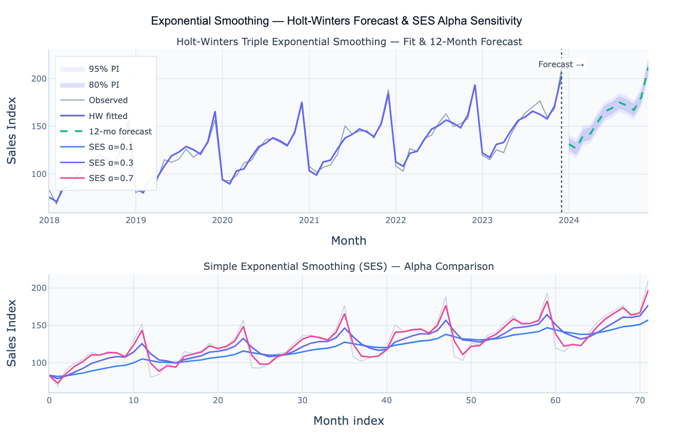
Exponential smoothing is a family of time series smoothing and forecasting methods that compute a weighted average of all past observations, with weights decreasing geometrically as observations get older. The smoothing equation is Sₜ = α · yₜ + (1 − α) · Sₜ₋₁, where α (alpha) is the smoothing parameter between 0 and 1: α close to 1 gives almost all weight to the most recent observation (fast-adapting, noisy); α close to 0 spreads weight broadly across history (slow-adapting, smooth). The resulting level Sₜ is both the smoothed representation of the current value and the one-step-ahead forecast. This simple form is called simple exponential smoothing (SES) or single exponential smoothing, and it is appropriate for stationary series with no systematic trend or seasonal pattern.
Holt's double exponential smoothing extends SES by adding a second equation that tracks the trend component separately, controlled by a second parameter β (beta). The level equation updates the current baseline; the trend equation updates the current slope. The forecast for h steps ahead is level + h × trend, projecting the current trend linearly into the future. Holt-Winters triple exponential smoothing adds a third component and parameter γ (gamma) for seasonality, producing a complete decomposition into level, trend, and seasonal components that can be either additive (seasonal amplitude is constant) or multiplicative (amplitude grows with the level). Holt-Winters is the workhorse of operational forecasting in retail, demand planning, and energy management — it handles trending, seasonal data with interpretable parameters and fast computation.
Parameter optimization is typically done by minimizing the sum of squared one-step-ahead forecast errors (SSE) over the historical data. The optimal α, β, and γ are the values that best balance smoothness against responsiveness in the specific dataset. A small α (0.05–0.2) indicates the series is smooth and level; a large α (0.6–0.9) indicates the series is noisy or changes rapidly. The fitted parameters are diagnostically meaningful: a large β means the trend changes quickly (non-linear); a large γ means the seasonal pattern shifts year to year.
How It Works
- Upload your data — provide a CSV or Excel file with a date column and a value column. Monthly, quarterly, or annual data all work. Seasonal data needs at least 2–3 full seasonal cycles. One row per time point.
- Describe the analysis — e.g. "Holt-Winters additive smoothing; optimize alpha, beta, gamma; 12-month forecast; 80% and 95% prediction intervals"
- Get full results — the AI writes Python code using statsmodels ExponentialSmoothing and Plotly to fit the model, produce in-sample fitted values, forecast with shaded prediction intervals, and report the smoothing parameters and error metrics
Required Data Format
| Column | Description | Example |
|---|---|---|
date | Date or timestamp | 2020-01, Jan 2020, 2020-01-31 |
value | Numeric time series | 245.3, 312.1, 198.8 (sales, temperature, etc.) |
Any column names work — describe them in your prompt. For seasonal Holt-Winters, specify the seasonal period (12 for monthly data, 4 for quarterly).
Interpreting the Results
| Parameter / Output | What it means |
|---|---|
| α (alpha) | Level smoothing — near 1 = reacts fast to new observations; near 0 = heavy historical averaging |
| β (beta) | Trend smoothing — near 1 = trend changes quickly; near 0 = slow-changing trend |
| γ (gamma) | Seasonal smoothing — near 1 = seasonal pattern updates rapidly year to year |
| In-sample RMSE / MAE | Average forecast error on training data — lower is better |
| AIC / BIC | Penalized goodness of fit — use to compare additive vs multiplicative models |
| Forecast | Point estimate for each future period based on projected level + trend + seasonal |
| Prediction interval | Range where future observations are expected to fall — widens with horizon |
| Additive vs multiplicative | Additive: seasonal amplitude is constant; multiplicative: amplitude grows with the level |
Example Prompts
| Scenario | What to type |
|---|---|
| Simple smoothing | SES with optimized alpha; overlay on raw data; what is the one-step-ahead forecast? |
| Holt trend | Holt double exponential smoothing; optimize alpha and beta; forecast 5 years; report trend slope |
| Holt-Winters forecast | Holt-Winters additive; seasonal period 12; optimize all parameters; 12-month forecast with 95% PI |
| Alpha sensitivity | SES with alpha = 0.1, 0.3, 0.5, 0.7; overlay all on raw data; which alpha minimizes RMSE? |
| Additive vs multiplicative | fit both additive and multiplicative Holt-Winters; compare AIC; which fits better? |
| Residual check | Holt-Winters fit; plot ACF of residuals; test if residuals are white noise (Ljung-Box test) |
Assumptions to Check
- Stationarity within model type — SES assumes no trend or seasonality; using SES on a strongly trending series produces forecasts that lag far behind; use Holt or Holt-Winters instead
- Additive vs multiplicative — if the seasonal amplitude grows proportionally with the level (percentage swings are constant), use multiplicative; if amplitude is constant in absolute terms, use additive; the model choice affects all three components
- Sufficient seasonal cycles — Holt-Winters requires at least 2 full seasonal cycles for seasonal parameter estimation; with fewer cycles the γ estimate is unreliable
- Outliers — exponential smoothing is not robust to outliers; a single extreme value permanently shifts the level component due to the recursive smoothing; detect and handle outliers before fitting
- Forecast horizon — exponential smoothing forecasts degrade with longer horizons because the uncertainty compounds; prediction intervals widen rapidly; treat long-horizon forecasts (> one seasonal cycle) with caution
Related Tools
Use the Moving Average Calculator for simpler non-forecasting smoothing (SMA, EMA) without the full forecasting framework. Use the Time Series Decomposition tool to formally extract trend, seasonal, and residual components for inspection before or instead of exponential smoothing. Use the Seasonality Analysis tool to characterize the seasonal pattern that Holt-Winters will capture. Use the Autocorrelation Plot (ACF) to check the residuals from an exponential smoothing fit — well-fitted residuals should show no ACF spikes.
Frequently Asked Questions
What is the difference between SES, Holt, and Holt-Winters?SES (one parameter α) is for stationary series — no trend, no seasonality. The forecast is a constant level. Holt (two parameters α, β) adds a trend component — the forecast is a straight line projected from the current level at the current slope. Holt-Winters (three parameters α, β, γ) adds a seasonal component — the forecast is a trended line modulated by the seasonal pattern. Choose based on what the data shows: if the series is flat, use SES; if it trends without seasonality, use Holt; if it has both trend and repeating cycles, use Holt-Winters.
How do I choose between additive and multiplicative Holt-Winters? Look at the seasonal amplitude over time. If December sales are always $50k above the annual average regardless of the overall sales level — the amplitude is constant — use additive. If December sales are always 30% above the annual average (the amplitude grows as total sales grow) — use multiplicative. A quick visual check: plot the series; if the peaks and troughs spread further apart as the series trends up, multiplicative is likely better. Quantitatively, fit both and compare AIC — the model with lower AIC is preferred. Ask the AI to "fit both additive and multiplicative Holt-Winters and compare AIC".
What does alpha = 0.3 mean in practical terms? With α = 0.3, the current observation contributes 30% of the new smoothed level; the previous smoothed level contributes 70%. Equivalently, the effective memory of the filter extends back roughly 1/α = 3.3 periods — the most recent 3–4 observations carry the majority of the weight. A smaller α (e.g. 0.05) spreads weight across 20 periods and changes slowly; a larger α (e.g. 0.8) reacts to the last 1–2 periods. The optimal α reflects the noise level: noisy series need smaller α for stability; rapidly changing series need larger α to stay current.
How are prediction intervals computed for exponential smoothing?
Prediction intervals for exponential smoothing are based on the forecast error variance, which grows with the forecast horizon. For SES, the h-step-ahead forecast variance is approximately σ² × (1 + (h−1)α²) where σ² is the one-step residual variance. The 95% PI is forecast ± 1.96 × RMSE × √(variance multiplier). Statsmodels computes these analytically with the simulate_smoother method. The intervals widen more steeply for larger α (more uncertainty per step) and less steeply for smaller α. Ask the AI to "plot 80% and 95% prediction intervals for the Holt-Winters forecast".