A/B Test Calculator for Conversion Experiments
Analyze A/B tests online from Excel or CSV data. Calculate conversion rates, lift, p-values, confidence intervals, and sample size checks with AI.
Or try with a sample dataset:
Preview
What Is an A/B Test?
An A/B test (also called a split test or controlled experiment) is a randomized experiment that compares two (or more) versions of a product, message, or intervention by exposing different groups of users to each version and measuring which performs better on a target metric. The core logic is identical to a clinical randomized controlled trial applied to digital products and marketing: the control group (A) receives the current version, the treatment group (B) receives the changed version, and outcomes (click-through rate, purchase conversion, sign-up rate, revenue) are compared after sufficient data has been collected. The statistical test determines whether the observed difference in performance could plausibly be explained by chance sampling variation or represents a genuine effect of the change.
For binary outcomes (converted / not converted), the appropriate test is the two-proportion z-test: it computes a z-statistic based on the observed proportions and their pooled standard error, then derives a p-value — the probability of observing a difference at least this large if the true conversion rates were equal. For continuous outcomes (revenue per user, time on page), a two-sample t-test is used instead. The relative lift — (p_B − p_A) / p_A × 100% — is the most business-relevant effect size: it expresses how much better (or worse) the variant performs relative to the control in percentage terms. A statistically significant test tells you the difference is unlikely due to chance; lift tells you the magnitude of the business impact.
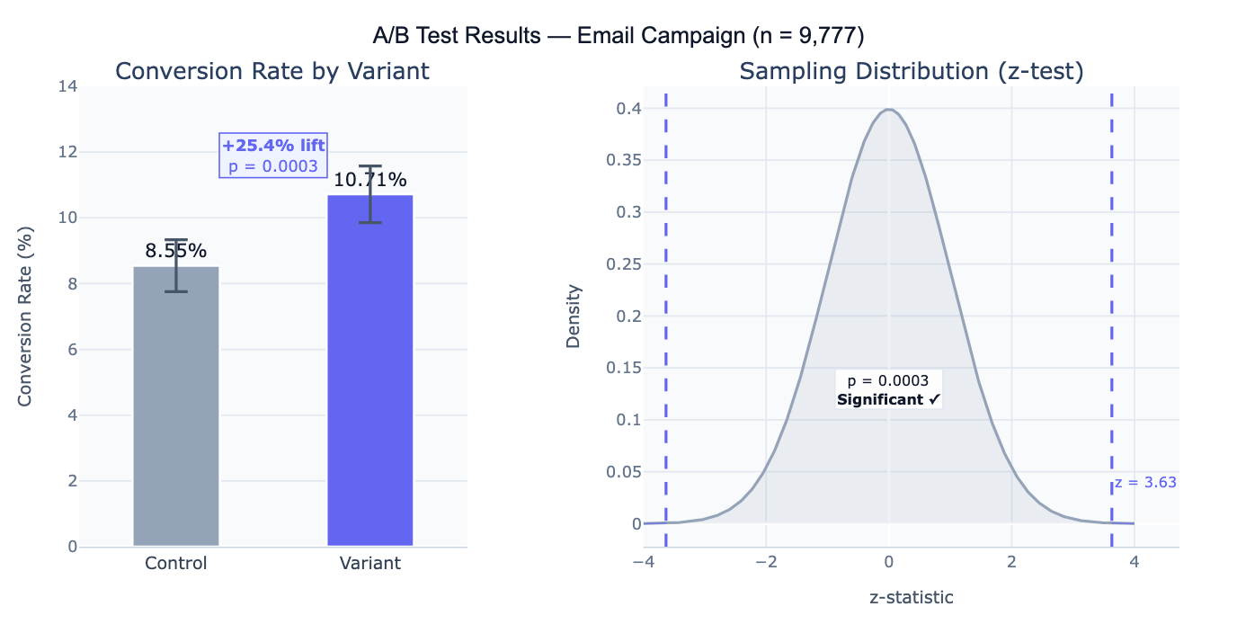
A concrete example: an e-commerce site tests a new checkout button color. Control: 4,821 users, 412 conversions (8.54%). Variant: 4,956 users, 531 conversions (10.71%). Lift = +25.4%, z = 3.63, p = 0.0003 — the result is highly significant. However, a critical follow-up question is whether the test was pre-registered with a predetermined sample size: if the team peeked at the data daily and stopped the test early when it looked significant, the reported p-value is invalid due to multiple looks (the "peeking problem"). Proper A/B testing requires deciding the sample size before running the test, based on the minimum detectable effect and desired power.
How It Works
- Upload your data — provide a CSV or Excel file with one row per user/observation, a column indicating the variant assignment (e.g.,
group: "control"/"variant"), and a column for the outcome (e.g.,converted: 0/1). Aggregate summaries (just counts and totals) can also be described directly in the prompt. - Describe the test — e.g. "control vs variant, binary conversion outcome in column 'converted', group column is 'group'; z-test for proportions; p-value, 95% CI, relative lift; bar chart; check if sample size was adequate for 80% power"
- Get full results — the AI writes Python code using scipy and Plotly to compute conversion rates, run the significance test, compute confidence intervals, and produce the conversion rate bar chart and sampling distribution visualization
Required Data Format
| Column | Description | Example |
|---|---|---|
group | Variant assignment | control, variant (or A, B) |
converted | Binary outcome | 1 (converted) or 0 (not converted) |
revenue | Optional: continuous outcome | 0, 29.99, 149.00 |
user_id | Optional: unique identifier | U12345 |
Any column names work — describe them in your prompt. For aggregate data (you only have totals, not individual rows), describe the numbers directly: "Control: 4821 users, 412 conversions; Variant: 4956 users, 531 conversions".
Interpreting the Results
| Output | What it means |
|---|---|
| Conversion rate (p_A, p_B) | Proportion of users who converted in each group |
| Absolute difference | p_B − p_A — the raw percentage point improvement |
| Relative lift | (p_B − p_A) / p_A × 100% — how much better the variant is relative to control |
| z-statistic | Test statistic comparing the two proportions under the null hypothesis of no difference |
| p-value | Probability of observing a difference this large if the null (no effect) is true — p < 0.05 is the conventional significance threshold |
| 95% CI on difference | Confidence interval for the true difference p_B − p_A — excludes 0 = significant |
| Statistical power | Probability the test would detect a true effect of the observed size (retrospective power) |
| Required sample size | N per group needed to detect a given minimum effect with target power |
Example Prompts
| Scenario | What to type |
|---|---|
| Basic conversion test | control vs variant, binary conversion column; z-test; p-value; relative lift; bar chart with 95% CI |
| Two-sided vs one-sided | one-sided z-test (variant > control); p-value for directional hypothesis; 95% one-sided CI |
| Continuous outcome | revenue per user is continuous; two-sample t-test; mean revenue by group; 95% CI on difference; Cohen's d effect size |
| Multiple variants (A/B/C) | 3 variants (A, B, C); pairwise z-tests; Bonferroni correction for multiple comparisons; adjusted p-values |
| Sample size check | was sample size adequate? compute minimum detectable effect at 80% power and α=0.05 given observed n |
| Pre-test power analysis | what sample size per group needed to detect 10% relative lift from baseline 8% conversion rate with 80% power? |
| Sequential testing | compute p-value at each week using group sequential testing (O'Brien-Fleming boundaries); plot alpha spending |
| Segmented analysis | run A/B test overall and separately by device (mobile vs desktop); check for heterogeneous treatment effects |
Assumptions to Check
- Randomization — users must be randomly and independently assigned to control or variant; if the same user can appear in both groups, or assignment was not random (e.g., all morning users got the variant), the test is invalid; check for sample ratio mismatch (SRM) — a significant chi-square test on the group sizes indicates a randomization failure
- No peeking / pre-specified sample size — the decision to stop the test must be made on pre-specified criteria, not by continuously monitoring the p-value and stopping when it drops below 0.05; repeated peeking inflates the Type I error rate substantially above the nominal α; if peeking is unavoidable, use sequential testing methods (O'Brien-Fleming, alpha spending) or Bayesian methods
- Stable unit treatment value assumption (SUTVA) — one user's exposure to the variant should not affect another user's outcome; violations occur in social networks (one user sees a variant and tells friends) or two-sided marketplaces (variant users compete with control users for the same inventory)
- Single metric focus — testing many metrics simultaneously without correction inflates false positives; designate one primary metric before running the test; secondary metrics require multiple comparison correction (Bonferroni, Benjamini-Hochberg)
- Novelty effect — a change in behavior due to users noticing something new (independent of its actual value) can create temporarily inflated treatment effects that fade over time; run the test for at least one full weekly cycle and monitor for effect decay
Related Tools
Use the Power Analysis Calculator to design the test before running it — determine the required sample size based on your baseline conversion rate, minimum detectable effect, significance level, and desired power. Use the Fisher's Exact Test Calculator for small-sample A/B tests (fewer than ~30 conversions per group) where the normal approximation underlying the z-test is unreliable. Use the Chi-Square Test Calculator for multi-variant tests (A/B/C/D) testing whether conversion rates differ across groups overall before running pairwise comparisons. Use the Logistic Regression calculator when you want to control for covariates (user demographics, device type, traffic source) in the A/B test analysis — regression-adjusted estimators can improve precision and account for imbalance.
Frequently Asked Questions
What p-value threshold should I use? The conventional threshold is α = 0.05 (5% false positive rate), but the right threshold depends on the stakes. For high-traffic tests where a wrong decision is cheap to reverse, α = 0.05 or even α = 0.10 may be appropriate to avoid slowing down iteration. For tests with large irreversible consequences (pricing changes, major product overhauls), α = 0.01 reduces false positives. The key insight is that p-value thresholds are a policy decision about the acceptable false positive rate, not a mathematical law — always consider the cost of a false positive (shipping a harmful change) versus a false negative (missing a real improvement) in context.
How long should I run the test? Run the test for at least the pre-specified duration determined by your sample size calculation — typically until you reach the target N per group. Never stop early just because the result looks significant (peeking problem) or because it has been running for a round number of days. As a minimum: (1) wait for at least one full business cycle (typically 1–2 weeks) to capture weekly seasonality in user behavior; (2) ensure you have reached the minimum detectable effect sample size before concluding no effect; (3) if you see the effect decaying over time, you may be observing a novelty effect rather than a real treatment effect.
My test is significant but the lift is tiny — should I ship it? Statistical significance and practical significance are separate questions. A very large sample can make even a 0.1% relative lift statistically significant (p < 0.05) when the true effect is negligibly small. Always evaluate results against a minimum detectable effect (MDE) that represents the smallest improvement worth the engineering cost of shipping the change. A useful rule of thumb: if the 95% confidence interval entirely falls below your MDE (even though it excludes 0), the test is statistically significant but practically inconclusive — the true effect is likely too small to matter. Report both the p-value and the confidence interval on the absolute and relative lift so stakeholders can make an informed decision.
What is a sample ratio mismatch (SRM) and why does it matter? An SRM occurs when the actual ratio of users in the control and treatment groups differs significantly from the intended ratio (e.g., you aimed for 50/50 but observed 48/52). SRMs are diagnosed with a chi-square goodness-of-fit test on group sizes. Common causes: logging bugs that miss events in one variant, bot filtering that affects groups differently, or assignment cache inconsistencies. SRM is critical to investigate before analyzing results because it indicates the randomization mechanism is broken — the groups are no longer comparable, and the estimated treatment effect is biased. Always check SRM before reporting A/B test results.