Statistical Power Analysis Calculator
Calculate sample size, effect size, and statistical power online for common study designs with AI.
Preview
What Is Power Analysis?
Statistical power is the probability that a study correctly detects a real effect when one exists — formally, power = 1 − β, where β is the probability of a Type II error (false negative: failing to detect a real effect). Power depends on four quantities that are linked by a mathematical relationship: sample size (n), effect size (δ), significance level (α), and power (1−β). Given any three of these, the fourth can be solved for. The most common use is a prospective power analysis: before data collection, fix the target power (conventionally 0.80 or 0.90), the acceptable false positive rate (α = 0.05), and the minimum effect size you care to detect, then calculate the required sample size. Underpowered studies waste resources and consistently fail to detect real effects; overpowered studies are wasteful; prospective power analysis finds the right balance.
The effect size is the magnitude of the phenomenon you want to detect, expressed in standardized units. For two independent means, Cohen's d = (μ₁ − μ₂) / σ — the difference in means divided by the pooled standard deviation. Conventions: d = 0.2 (small), d = 0.5 (medium), d = 0.8 (large). For proportions, use Cohen's h; for correlations, use r directly; for chi-square, use Cramér's V; for ANOVA, use Cohen's f. The effect size should ideally come from a pilot study, a published meta-analysis, or the minimum clinically meaningful difference — not from the first study's result, which inflates the estimate due to winner's curse.
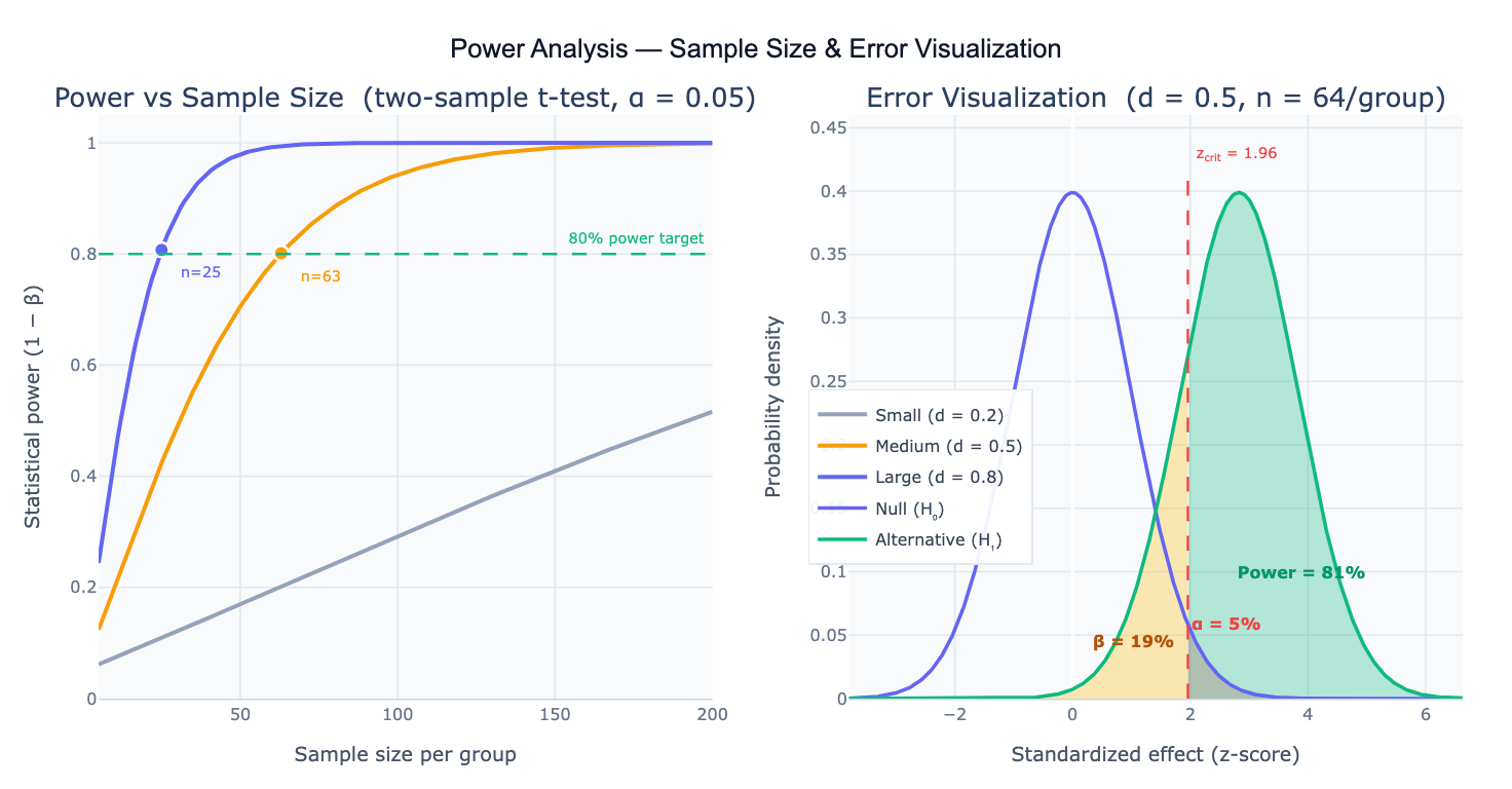
A Type I error (false positive) occurs with probability α — concluding an effect exists when it doesn't. A Type II error (false negative, β) occurs when a real effect is missed. The two distributions in the power diagram — the null distribution centered at zero and the alternative distribution shifted by the effect size — illustrate these geometrically: the red tail of the null distribution to the right of the critical value is α; the green tail of the alternative distribution to the right of the critical value is power; the yellow region of the alternative distribution below the critical value is β. Power increases as the two distributions separate further — i.e., as effect size increases or sample size grows (reducing the standard error and narrowing both distributions).
How It Works
- Describe the analysis — specify your statistical test, the effect size (or the raw parameters to compute it), the significance level α, and what you want to solve for (usually sample size given target power, or power given existing sample size)
- Get full results — the AI writes Python code using scipy.stats and statsmodels.stats.power to solve the power equation, then generates power curves and the two-distribution diagram with labeled α, β, and power regions
No data upload required — power analysis is a prospective planning calculation based on the design parameters you specify.
Interpreting the Results
| Output | What it means |
|---|---|
| Required n | Minimum sample size per group (or total) to achieve the target power |
| Achieved power | Power at the specified n — compare to your target (usually 0.80 or 0.90) |
| Effect size | Standardized magnitude — Cohen's d, f, h, w, or r depending on the test |
| α (alpha) | Probability of a false positive — conventionally 0.05; use 0.01 for stricter control |
| β (beta) | Probability of a false negative = 1 − power; conventionally ≤ 0.20 |
| Power curve | Power vs sample size plot — shows how quickly power accumulates and the steep initial gains from adding participants |
| Distribution diagram | Null and alternative distributions with critical value; red = α, yellow = β, green = power |
| Sensitivity analysis | Power at different n values or effect sizes — useful when exact effect size is uncertain |
Example Prompts
| Scenario | What to type |
|---|---|
| Two-sample t-test | two-sample t-test, Cohen's d = 0.5, alpha = 0.05, power = 0.80 — required sample size per group? |
| One-sample t-test | one-sample t-test, expected mean = 105, null mean = 100, SD = 15, alpha = 0.05, power = 0.90 |
| Paired t-test | paired t-test for before/after design, mean difference = 8, SD of differences = 20, alpha = 0.05, target power = 0.80 |
| Chi-square test | chi-square test of independence, expected proportions 0.3 vs 0.5, alpha = 0.05, power = 0.80 |
| One-way ANOVA | one-way ANOVA with 4 groups, Cohen's f = 0.25 (medium effect), alpha = 0.05, power = 0.80 |
| Correlation | test Pearson correlation r = 0.3, alpha = 0.05, power = 0.80 — required n? |
| Post-hoc power | I have n=45 per group, two-sample t-test, alpha = 0.05, Cohen's d = 0.4 — what power did I achieve? |
| Effect size from data | mean1 = 12.3, mean2 = 10.5, pooled SD = 4.2; compute Cohen's d; then find n for 80% power at alpha = 0.05 |
| Power curve | plot power vs sample size for Cohen's d = 0.2, 0.5, 0.8; two-sample t-test; alpha = 0.05; mark 80% and 90% power lines |
| Survival study | log-rank test power; control median survival 12 months, treatment 18 months, exponential survival; 1:1 allocation; alpha = 0.05, power = 0.80 |
Frequently Asked Questions
Why is 80% power the conventional standard? The 80% convention was popularized by Jacob Cohen in his 1977 book Statistical Power Analysis for the Behavioral Sciences, where he argued that a Type II error (missing a real effect) is roughly 4× less costly than a Type I error (falsely claiming an effect), making a 4:1 ratio of α:β (0.05:0.20 → power = 0.80) a reasonable default. This is a pragmatic heuristic, not a universal law — clinical trials often require 90% power to reduce the risk of failing to detect a clinically important treatment benefit; exploratory research may accept 70% power when resources are constrained; regulatory submissions may require 90–95% power for primary endpoints. Set your power target based on the consequences of missing the effect, not just convention.
What effect size should I use? Use the minimum effect size of practical interest — the smallest effect that would change your decision or be meaningful to the field. Do not use the effect size from a pilot study naively: small pilot studies produce highly variable effect size estimates, and using a lucky large pilot estimate will produce an underpowered main study (the "winner's curse"). Better sources: (1) published meta-analyses in your area; (2) clinically defined minimum important differences (e.g., a 5-point change on a 0–100 scale); (3) Cohen's conventions (d = 0.2/0.5/0.8 for small/medium/large) as a last resort when no prior data exists. When uncertain, run a sensitivity analysis: compute required n across a range of plausible effect sizes and plan for the most conservative estimate.
What is the difference between one-tailed and two-tailed power analysis? A two-tailed test (the default) tests whether μ₁ ≠ μ₂ — the effect could be in either direction. A one-tailed test tests whether μ₁ > μ₂ (or < μ₂ specifically). For the same α, a one-tailed test places the entire rejection region in one tail, making it easier to reject the null (lower required n for the same power). One-tailed tests are only appropriate when the effect can logically only occur in one direction and this direction is specified before data collection. Using a one-tailed test post-hoc to rescue a marginally significant result is not valid. For most research, use two-tailed tests.
How do I account for dropout or missing data in sample size calculation? Calculate the required sample size for complete data, then inflate by the expected dropout fraction: n_enrolled = n_complete / (1 − dropout_rate). For example, if 80 completers are needed and you expect 20% dropout, enroll 80 / 0.8 = 100 participants. For longitudinal studies or clinical trials with multiple time points, the dropout adjustment compounds and may require modeling (e.g., for repeated-measures ANOVA, the power calculation must account for the correlation structure among time points, not just the marginal sample size). Ask the AI to "adjust sample size for 25% expected dropout; required completers = 64".
My observed effect size is much smaller than my power analysis assumed — what should I do? This is common and has two causes: (1) winner's curse — the pilot or literature estimate was inflated by publication bias or small-sample variability; (2) the true effect is genuinely smaller than anticipated. Options: (1) report the post-hoc power for the observed effect (this is informative for future studies, though it should not be used to conclude "no effect"); (2) pool your data in a meta-analysis with other studies; (3) pre-register a larger replication; (4) use equivalence testing (TOST) if you want to formally demonstrate that the effect is smaller than a meaningful threshold. Avoid using observed power to justify a non-significant result — an underpowered study's null result is uninformative, not evidence of absence.