Melt Curve Analysis
Analyze qPCR melt curves online from Excel or CSV data. Detect Tm, identify nonspecific products, and compare peak profiles with AI.
Preview
What Is Melt Curve Analysis?
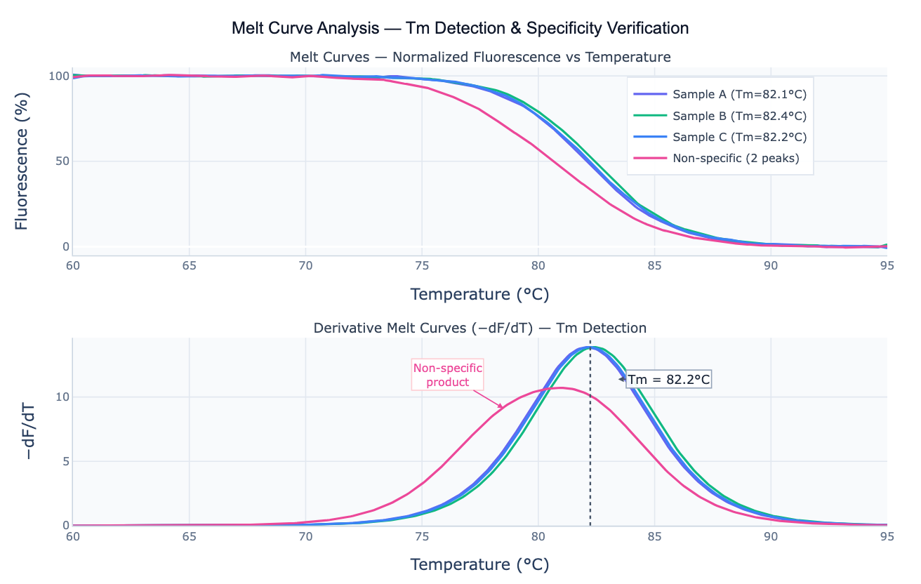
Melt curve analysis (also called dissociation curve analysis) monitors the fluorescence of a double-stranded DNA product as the temperature is raised from approximately 60°C to 95°C at the end of a qPCR run. Double-stranded DNA intercalates fluorescent dye (SYBR Green or similar); as the temperature rises and the two strands separate (denature), fluorescence drops sharply at the melting temperature Tm — the temperature at which 50% of the duplex is single-stranded. The Tm is characteristic of the PCR product's length and GC content, making it a specific identifier for each amplicon. A single, sharp sigmoidal fluorescence drop produces a single sharp peak in the derivative melt curve (−dF/dT), confirming that only one PCR product was amplified.
The primary purpose of melt curve analysis is product specificity verification. If primers amplify the intended target only, all wells containing the same amplicon will produce identical, reproducible Tm values within ±0.5°C, and the derivative curve shows a single symmetric peak. If non-specific amplification has occurred (primer dimers, off-target products), the derivative curve shows multiple peaks at different temperatures — often a lower-Tm shoulder from primer dimers (~72–78°C) alongside the main product peak. A broad or asymmetric single peak suggests heterogeneous products or template contamination. Melt curve analysis is therefore a mandatory quality control step for every SYBR Green qPCR assay, run automatically at the end of every PCR cycle protocol.
High-resolution melt (HRM) extends standard melt curve analysis to genetic applications: with high-precision thermal cyclers (±0.02°C resolution) and saturating dyes, small differences in melting profile reveal single-nucleotide polymorphisms (SNPs), methylation status differences, and copy number variants without sequencing. HRM normalizes the raw fluorescence curves to a common pre- and post-melt baseline, then clusters samples by curve shape — heterozygous SNP carriers produce distinctly shaped curves that separate clearly from homozygous wild-type and variant samples. The derivative Tm of heterozygous samples shifts by 0.5–1.5°C relative to homozygous samples, and the curve shape shows a characteristic shoulder or inflection.
How It Works
- Upload your data — provide a CSV or Excel file with a temperature column and one column of fluorescence per sample (or a long-format file with sample and fluorescence columns). One row per temperature step.
- Describe the analysis — e.g. "plot derivative melt curves for all samples; identify Tm for each; flag any sample with multiple peaks; compare Tm between groups"
- Get full results — the AI writes Python code using scipy.signal.savgol_filter for smooth derivative computation, scipy.signal.find_peaks for Tm detection, and Plotly to render normalized melt curves, derivative plots, and a Tm summary table
Required Data Format
| Column | Description | Example |
|---|---|---|
temperature | Temperature in °C | 60.0, 60.2, 60.4 … 95.0 |
sample_1, sample_2, … | Fluorescence for each well | 8245, 8210, 7980 … (raw RFU) |
Alternatively, use long format: one row per temperature–sample pair with columns temperature, sample, fluorescence. Any column names work — describe them in your prompt.
Interpreting the Results
| Output | What it means |
|---|---|
| Tm | Melting temperature — peak of −dF/dT; characteristic of amplicon length and GC content |
| Single peak | One PCR product — assay is specific; the Tm confirms product identity |
| Two peaks | Two products — often main amplicon + primer dimer (lower Tm ~72–78°C) or off-target |
| Broad peak | Heterogeneous products or poor primer design — investigate primer specificity |
| Tm shift between samples | Different products (HRM: SNP/mutation) or pipetting/template contamination |
| Normalized fluorescence | Pre-melt = 100%, post-melt = 0%; normalization allows shape comparison across wells |
| Tm CV (%) | Coefficient of variation across replicates — should be < 0.5°C for a clean assay |
| Negative control peak | Fluorescence in the no-template control at ≤ 78°C = primer dimer only (acceptable if below main product Tm) |
Example Prompts
| Scenario | What to type |
|---|---|
| Basic QC | plot normalized melt curves and derivative (−dF/dT) for all samples; identify Tm for each; flag samples with multiple peaks |
| Tm table | extract Tm from each derivative peak; report mean Tm, SD, and CV across replicates; flag outliers > 1°C from mean |
| Specificity check | identify samples with double peaks (non-specific amplification); list their well IDs and secondary peak temperatures |
| HRM genotyping | normalize melt curves; cluster samples by curve shape; identify putative SNP variants from Tm shift and curve shape difference |
| Primer dimer check | plot negative control melt curve; report Tm of any peaks; confirm primer dimer Tm is below main product Tm |
| Group comparison | compare Tm between 'treated' and 'control' groups in the 'group' column; t-test for Tm difference; plot side-by-side |
Assumptions to Check
- Correct temperature range — the temperature program should start below Tm − 10°C and end above Tm + 5°C to fully capture the sigmoidal transition; truncated data misses the baseline and distorts normalization
- Smooth ramp rate — steep temperature ramps (> 0.5°C/s) produce noisy melt curves; most instruments use 0.1–0.2°C/s for SYBR melt curves and 0.01–0.05°C/s for HRM
- Baseline fluorescence — pre-melt fluorescence should be stable (flat plateau); a rising baseline indicates incomplete extension in the final cycle; a falling baseline may indicate photobleaching
- Normalization required for HRM — raw fluorescence comparison is unreliable; normalize each curve to a common pre-melt (100%) and post-melt (0%) baseline before shape comparison or clustering
- Single product assumption — standard Tm interpretation assumes one dominant product; if two products are present with similar Tm, they may produce a single broad peak that appears specific — always confirm with gel electrophoresis for critical assays
Related Tools
Use the qPCR Standard Curve Calculator to calculate PCR efficiency, R², and quantify unknown samples from Ct values. Use the Peak Finder to automatically detect Tm peaks in derivative melt curves when analyzing many samples programmatically. Use the Gaussian Peak Fit to fit parametric Gaussian models to derivative melt curve peaks for precise Tm with confidence intervals. Use the Clustergram Generator to cluster and visualize normalized HRM curves across many samples as a heatmap.
Frequently Asked Questions
What is the difference between a raw melt curve and a derivative melt curve? The raw melt curve plots fluorescence (RFU) vs temperature — it shows a sigmoidal drop from high (fully double-stranded) to near zero (fully single-stranded). The derivative melt curve (−dF/dT) plots the negative rate of fluorescence change vs temperature — it converts the sigmoidal drop into a peak whose apex is the Tm. Derivative curves are preferred because: (1) the peak position is more precise than estimating the midpoint of a sigmoid; (2) multiple products appear as separate peaks; (3) peak width reports on product homogeneity. Always inspect both — the raw curve reveals baseline issues that the derivative might obscure.
My negative control (NTC) has a peak around 72–76°C — is this normal? A low-temperature peak in the NTC (72–78°C) is almost always primer dimers — short duplexes formed between the primers themselves. Primer dimers are normal at low levels and are acceptable as long as: (1) their Tm is clearly below the main product Tm (separated by ≥ 4°C); (2) the NTC Ct is much higher than the sample Ct (typically undetermined or > 35); (3) the NTC shows no peak at the main product Tm. If the NTC shows a peak at the same Tm as your samples, you have template contamination and the run is invalid.
How do I identify a non-specific product vs primer dimer by melt curve?Primer dimers typically melt at 72–78°C (short, low-GC duplexes). Non-specific amplification (off-target product) melts at a different temperature than the intended amplicon but is usually within 5°C of it (75–82°C for typical genomic targets). If a second peak is below 78°C, it is almost certainly primer dimers. If it is within 2–5°C of the main product, it is likely an off-target amplification — redesign the primers or increase the annealing temperature. Ask the AI to "plot derivative melt curves; classify any second peaks as primer dimer (Tm < 78°C) or non-specific product (Tm > 78°C); list affected wells".
Can melt curve analysis replace gel electrophoresis for product verification? Melt curve analysis is faster and higher-throughput than gel electrophoresis but is not a complete replacement. Melt analysis confirms that a product exists at a specific Tm — but two different sequences of similar length and GC content can have nearly identical Tm values. Gel electrophoresis confirms product size, which melt analysis cannot. For a new primer pair being validated for the first time, always confirm with gel electrophoresis. For routine use of an established, validated assay, melt curve analysis alone is sufficient for product specificity QC.