qPCR Standard Curve Calculator
Analyze qPCR standard curves online from Excel or CSV data. Calculate PCR efficiency, slope, R-squared, and unknown sample quantities with AI.
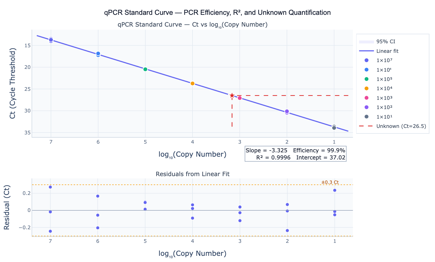
Preview
What Is a qPCR Standard Curve?
A qPCR standard curve (quantitative PCR standard curve) is a linear regression of Ct (cycle threshold) values against the log₁₀ of template concentration or copy number for a series of serial dilutions of a known reference material. Because PCR amplification is exponential, a 10-fold dilution produces a Ct increase of approximately 3.32 cycles (at 100% efficiency), making the relationship between Ct and log₁₀concentration precisely linear. The slope of this line is the primary quality indicator: an ideal slope of −3.32 corresponds to exactly 100% PCR efficiency (perfect doubling per cycle); slopes between −3.1 and −3.6 (efficiency 90–110%) are considered acceptable by most guidelines (MIQE).
The PCR efficiency is calculated from the slope as E = (10^(−1/slope) − 1) × 100%. A slope of −3.32 gives E = 100%; −3.58 gives ~90%; −3.10 gives ~110%. Values outside 90–110% indicate inhibition (too shallow a slope, E < 90%) or pipetting errors, primer dimers, or non-specific amplification (too steep, E > 110%). The R² (coefficient of determination) must be ≥ 0.98 for a reliable standard curve; R² < 0.98 indicates inconsistent replicates, pipetting error, or a non-linear relationship. Together, slope, efficiency, and R² are the three mandatory quality metrics reported in every qPCR publication.
Once validated, the standard curve is used to quantify unknown samples: measure their Ct values and back-calculate concentration as C = 10^((Ct − intercept) / slope). The intercept determines the detection limit — a higher intercept means the assay detects lower template amounts. Standard curves should be run in the same qPCR plate as unknowns to control for run-to-run variation in amplification efficiency. For multi-gene relative quantification (ΔΔCt method), separate standard curves must be validated for both the target gene and the reference gene to confirm comparable efficiencies.
How It Works
- Upload your data — provide a CSV or Excel file with a concentration column (template copies or dilution factor) and a Ct column. Include a replicate column if you have multiple replicates per dilution. One row per well.
- Describe the analysis — e.g. "fit standard curve; calculate efficiency, slope, R²; quantify unknown samples with Ct values 28.5, 30.2, 31.0; plot residuals"
- Get full results — the AI writes Python code using scipy.stats.linregress and Plotly to fit the standard curve, report all quality metrics, annotate unknown sample concentrations on the curve, and produce a residual plot
Required Data Format
| Column | Description | Example |
|---|---|---|
concentration | Template copies or dilution fold | 1e7, 1e6, 1e5, 1e4, 1e3 |
ct | Cycle threshold value | 12.3, 15.6, 18.9, 22.1, 25.4 |
replicate | Optional: replicate number | 1, 2, 3 |
sample | Optional: sample or gene label | GAPDH, TargetGene |
Any column names work — describe them in your prompt. Concentrations can be input as copy numbers, ng/µL, dilution factors (1:10, 1:100), or log₁₀ values.
Interpreting the Results
| Output | What it means |
|---|---|
| Slope | Should be −3.32 (100% efficiency); acceptable range −3.1 to −3.6 |
| PCR efficiency (%) | E = (10^(−1/slope) − 1) × 100; acceptable 90–110% |
| R² | Linearity — must be ≥ 0.98; < 0.98 indicates pipetting errors or inhibition |
| Intercept | Ct at 1 copy (or 1 ng); higher intercept = less sensitive assay |
| 95% confidence interval on slope | Precision of efficiency estimate — wide CI = few replicates or high variability |
| Quantified unknown C | C = 10^((Ct − intercept) / slope) — back-calculated from the standard curve |
| Residuals | Should be random scatter within ±0.3 Ct; patterned residuals = non-linearity |
| LOD / LOQ | Lowest Ct where signal is reliably above background; estimated from the lowest standard point |
Example Prompts
| Scenario | What to type |
|---|---|
| Basic standard curve | fit standard curve to Ct vs log10(copies); report slope, efficiency, R²; plot with 95% CI band |
| Quantify unknowns | standard curve with dilutions 1e7 to 1e2; quantify unknown samples with Ct values 25.1, 27.4, 30.0 |
| Multi-gene comparison | fit standard curves for GAPDH and TargetGene; compare efficiencies; confirm ΔΔCt method is valid (efficiencies within 5%) |
| Replicate analysis | 3 technical replicates per standard; plot individual points and mean; flag outlier replicates (ΔCt > 0.5) |
| Residual check | standard curve fit; plot residuals vs log concentration; test for systematic non-linearity |
| Report generation | standard curve analysis; produce full MIQE-compliant summary table with slope, efficiency, R², intercept, and 95% CI |
Assumptions to Check
- Minimum 5 dilution points — a reliable standard curve requires at least 5 points spanning at least 4 log units; fewer points or a narrower range increases uncertainty on slope and efficiency
- Triplicates per dilution — technical triplicates are the standard minimum; duplicates are acceptable for exploratory work but reduce statistical power
- Linearity over the full range — if the highest concentrations show plateau (late log-phase inhibition) or the lowest show increased variability (approaching LOD), these points should be excluded; test linearity with the residual plot
- Same plate as unknowns — standard curves should ideally run on the same plate as unknown samples; inter-run efficiency variation can introduce systematic error if curves from different runs are used
- No reverse transcription variation — for RT-qPCR, the standard curve quantifies after RT; variation in reverse transcription efficiency between samples is not captured by the standard curve and must be controlled separately
Related Tools
Use the Linear Regression tool when you need general linear regression outside of the qPCR context — standard curve fitting is a special case of linear regression. Use the Dose-Response Curve Generator for sigmoidal inhibition or activation curves in pharmacology. Use the Residual Plot Generator to inspect standard curve residuals in detail and test for systematic non-linearity.
Frequently Asked Questions
What is PCR efficiency and why does it matter?PCR efficiency measures how well the polymerase doubles the template at each cycle. At 100% efficiency (slope = −3.32), the template exactly doubles each cycle; at 80% efficiency (slope = −3.74), only 1.8-fold amplification occurs per cycle. Efficiency < 90% indicates inhibitors (salts, EDTA, heparin, humic acids), suboptimal primer design, or inefficient annealing temperature. For absolute quantification, the standard curve corrects for efficiency automatically. For relative quantification (ΔΔCt), the Livak method assumes equal efficiency for target and reference genes — efficiency differences of > 5% invalidate the simplified 2^(−ΔΔCt) formula and require the Pfaffl method instead.
My R² is 0.997 but one dilution point looks off — should I remove it? Removing a point to improve R² is only justified if there is an independent technical reason (documented pipetting error, visible contamination, outlier replicate > 0.5 Ct from the other two replicates at the same dilution). Removing points solely to improve statistics is data manipulation. Instead: (1) check if all replicates at that dilution are consistently offset (a dilution error) or only one replicate is off (a pipetting error); (2) rerun the standard curve; (3) if the point is legitimately excluded, document the reason in the methods.
How do I quantify an unknown sample below the lowest standard? Extrapolation below the lowest standard is unreliable — the efficiency may change near the detection limit, and stochastic amplification introduces noise. Best practice: include a standard at the expected concentration range of your unknowns; if unknowns are below the lowest standard, the result should be reported as below the limit of quantification (LOQ) or the assay should be re-run with a lower dilution series. The LOQ is typically defined as the lowest standard with CV < 25% across replicates and > 3× signal above the no-template control.
Should I use absolute copy number or relative dilution as the x-axis? Both work mathematically — the slope and R² are identical regardless of which unit is on the x-axis. Copy number (molecules per µL) is preferred for absolute quantification (reporting copies per sample); it requires a quantified reference material (e.g. plasmid or synthetic RNA with a known concentration). Dilution factor (10⁻¹, 10⁻², …) is acceptable for relative quantification where only efficiency and linearity matter. Describe your units clearly in the prompt so the AI labels the axes correctly and applies the right back-calculation formula.
qPCR Efficiency Calculator
qPCR efficiency (also called amplification efficiency or primer efficiency) quantifies how effectively the PCR reaction doubles the template DNA at each cycle. To calculate qPCR efficiency from a standard curve, upload your Ct vs log₁₀concentration data and prompt:
"fit standard curve; calculate PCR efficiency from slope using E = (10^(−1/slope) − 1) × 100; report efficiency, slope, and R²; plot standard curve with equation"
The AI fits the linear regression and automatically computes the efficiency. Acceptable qPCR efficiency range is 90–110%. Efficiency outside this range indicates assay problems: below 90% suggests PCR inhibitors or poor primer design; above 110% suggests primer dimers, non-specific amplification, or pipetting errors.
| Slope | Efficiency | Interpretation |
|---|---|---|
| −3.10 | 110% | Too high — primer dimers or non-specific amplification |
| −3.32 | 100% | Ideal — template perfectly doubles each cycle |
| −3.45 | 95% | Acceptable |
| −3.58 | 90% | Lower acceptable limit |
| −3.74 | 85% | Too low — inhibition likely |
| −4.00 | 78% | Unacceptable — assay must be re-optimized |
PCR Efficiency Formula
The PCR efficiency formula derived from the standard curve slope is:
E (%) = (10^(−1/slope) − 1) × 100
Where slope is the slope of the linear regression of Ct versus log₁₀(template concentration). This formula comes from the exponential amplification model: at each cycle, the amount of product is multiplied by (1 + E/100). A 10-fold dilution of template increases the Ct by 1/log₁₀(1 + E/100) cycles — which equals exactly 3.32 cycles at 100% efficiency. Rearranging: slope = −1/log₁₀(1 + E/100), so E = (10^(−1/slope) − 1) × 100.
To apply the formula manually from a reported slope: if your slope is −3.45, then E = (10^(−1/−3.45) − 1) × 100 = (10^0.290 − 1) × 100 = (1.95 − 1) × 100 = 95%.
Ask the AI to "compute PCR efficiency from slope −3.45 using the formula E = (10^(−1/slope) − 1) × 100; show the calculation step by step".
Primer Efficiency qPCR
Primer efficiency in qPCR is the same as PCR amplification efficiency — it measures how well a specific primer pair amplifies its target under the chosen reaction conditions. Each primer pair has its own efficiency, which depends on primer sequence, GC content, secondary structure, annealing temperature, and Mg²⁺ concentration. A primer pair with 95% efficiency amplifies the target ~1.95-fold per cycle instead of the ideal 2-fold.
For relative quantification using the ΔΔCt method (Livak method), both the target gene and the reference gene must have primer efficiencies within 5% of each other (ideally within 2%). If efficiencies differ by more than 5%, the simplified 2^(−ΔΔCt) formula systematically overestimates or underestimates the fold change — the Pfaffl method must be used instead, which corrects for efficiency differences: Ratio = (E_target)^ΔCt_target / (E_reference)^ΔCt_reference.
To validate primer pairs: run a standard curve for each gene, calculate efficiency, and prompt: "compare primer efficiencies for GAPDH and TargetGene; confirm they are within 5% for ΔΔCt validity; if not, compute fold change using the Pfaffl correction".