Lead Scoring Model Calculator
Build lead scoring models online from Excel or CSV CRM data. Rank prospects, score conversion probability, and evaluate model quality with AI.
Or try with a sample dataset:
Preview
What Is a Lead Scoring Model?
A lead scoring model assigns each prospect a numeric score — typically 0 to 100 — representing their estimated probability of converting to a customer, patient, student, or program participant. Rather than treating all leads equally or relying on intuition, a data-driven scoring model learns from historical conversions: it identifies which observable characteristics (job title, company size, behavioral signals like demo requests or page visits) are most predictive of conversion and combines them into a single actionable score. Sales and marketing teams use these scores to prioritize outreach — focusing effort on high-score "hot leads" where conversion probability is highest, and deprioritizing low-score leads that are unlikely to convert regardless of effort invested.
The statistical foundation is logistic regression (or a gradient-boosted classifier for non-linear patterns), which models the log-odds of conversion as a linear combination of input features. Each feature receives a coefficient — a positive coefficient means more of that feature increases conversion probability, a negative coefficient means it decreases it. The raw predicted probability (0 to 1) is multiplied by 100 to produce the 0–100 lead score. Feature importance (the magnitude of each coefficient) reveals which signals matter most: in a B2B context, a demo request might have a coefficient of +1.8 (strongly predictive), while website visits might add only +0.05 per visit. Understanding feature importance is often as valuable as the scores themselves — it tells the marketing team which engagement signals to invest in creating.
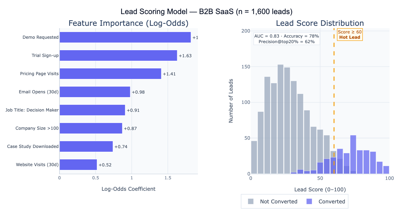
A concrete example: a B2B SaaS company builds a scoring model on 1,600 historical leads (320 converted, 1,280 did not). The model achieves AUC = 0.83, meaning it correctly ranks a randomly chosen converter above a non-converter 83% of the time. Setting a threshold at score ≥ 60, the top 20% of leads capture 62% of all conversions — the sales team can focus on 320 "hot leads" and close 3× as many deals per call as they would working the full list. The feature importance chart shows that "Demo Requested" (+1.82) and "Trial Sign-up" (+1.63) are the strongest predictors, suggesting that the highest-ROI marketing investment is driving prospects to request demos or start trials.
How It Works
- Upload your data — provide a CSV or Excel file with one row per lead, a binary outcome column (1 = converted, 0 = did not convert), and feature columns representing lead characteristics and behaviors.
- Describe the model — e.g. "outcome = converted, features = company_size, job_title, page_visits, email_opens, demo_requested; logistic regression; score 0–100; feature importance; AUC; precision at top 20%"
- Get full results — the AI writes Python code using scikit-learn and Plotly to train the model, compute scores for all leads, plot feature importance, produce the ROC curve, and output a ranked lead list
Required Data Format
| Column | Description | Example |
|---|---|---|
converted | Binary outcome | 1 (converted) or 0 (did not) |
company_size | Numeric or categorical feature | 250, enterprise, SMB |
job_title | Lead characteristic | VP Sales, Engineer, CEO |
page_visits | Behavioral signal | 12, 3, 0 |
email_opens | Engagement feature | 5, 0, 18 |
demo_requested | Binary flag | 1, 0 |
Any column names work — list the features and outcome in your prompt. Categorical features (job title, industry) are automatically one-hot encoded. Missing values are imputed with column medians/modes. More rows (> 500 with both outcomes) produce more reliable models.
Interpreting the Results
| Output | What it means |
|---|---|
| Lead score (0–100) | Each lead's estimated conversion probability × 100 — higher = more likely to convert |
| Feature importance | Log-odds coefficient for each feature — magnitude shows importance, sign shows direction |
| AUC (ROC curve) | Area under the ROC curve — 0.5 = no better than random, 1.0 = perfect ranking; 0.70–0.85 is typical for lead scoring |
| Precision at top N% | What fraction of the top-scoring N% leads actually converted — the most business-relevant metric |
| Threshold recommendation | Score cutoff that optimizes the precision/recall trade-off for a given sales capacity |
| Score distribution | Histogram of scores for converted vs non-converted leads — good separation means the model is predictive |
| Ranked lead list | All leads sorted by score — ready to export to CRM for prioritized outreach |
| Lift curve | Ratio of model precision to random baseline — e.g., "top 20% of scored leads are 3× more likely to convert" |
Example Prompts
| Scenario | What to type |
|---|---|
| Basic scoring | outcome = converted; features = company_size, visits, email_opens; logistic regression; score 0–100; feature importance; AUC |
| Threshold setting | at what score threshold does precision reach 50%? compute precision and recall at score = 40, 50, 60, 70, 80 |
| Top-N analysis | what % of conversions are captured in the top 10%, 20%, 30% of leads by score? lift chart |
| Segment scores | compute average lead score by industry and job title; which segments score highest? |
| Model comparison | compare logistic regression vs random forest for lead scoring; AUC comparison; feature importance for both |
| Score calibration | plot calibration curve: do predicted probabilities match observed conversion rates? calibrate if necessary |
| Negative signals | which features reduce conversion probability? show negative coefficients; are there any surprising negative predictors? |
| Score over time | plot average lead score by lead acquisition month; is lead quality improving or declining? |
Assumptions to Check
- Representative training data — the model learns from historical conversions; if past conversions were influenced by sales capacity constraints (sales only called certain leads, so other leads never had a chance to convert), the model learns biased conversion signals; this is called survivorship bias and leads to underscoring leads that were never contacted
- Sufficient positive examples — logistic regression requires a reasonable number of conversions in the training data; with fewer than 50 conversions, the model is likely overfit and unstable; aim for at least 100–200 positive cases; with very few conversions, consider regularization (ridge penalty) or simpler models
- Feature relevance stability — the model assumes that the features that predicted conversion historically will continue to predict it in the future; if the market or product changes significantly, retrain the model on recent data rather than relying on a model trained on historical behavior
- No data leakage — features must reflect information available at the time of scoring, not information that is only known after the conversion decision (e.g., "meeting held" or "proposal sent" should only be used if they occur before the conversion event being predicted); leakage inflates AUC and produces scores that cannot be used in practice
- Class imbalance — if conversions are rare (< 5% of leads), the model may achieve high accuracy by predicting "no conversion" for everyone; check precision and recall rather than accuracy; use class-weight balancing or oversampling techniques if imbalance is severe
Related Tools
Use the Logistic Regression calculator to build the underlying classification model and examine the full regression output with p-values and confidence intervals on each feature coefficient. Use the ROC Curve and AUC Calculator to evaluate model discrimination performance and compare multiple scoring models — AUC is the primary metric for ranking-based lead scoring. Use the Confusion Matrix & Sensitivity Specificity Calculator to evaluate precision, recall, and F1-score at the chosen score threshold — different thresholds optimize for different business objectives (high precision vs. high recall). Use the A/B Test Calculator to test whether routing high-scoring leads to a specialized sales team significantly improves conversion rates compared to standard routing. Use the Conversion Funnel Analysis to analyze how scored leads flow through the sales pipeline stages — do high-scoring leads advance further in the funnel even when they ultimately don't convert?
Frequently Asked Questions
Should I use logistic regression or a machine learning model like random forest?Logistic regression is the right choice when interpretability matters — you need to explain to sales why a lead scores high or low, and the feature importance coefficients are directly interpretable. It works well for up to 20–30 features and typically achieves AUC = 0.70–0.80 for standard lead data. Random forest or gradient boosting (XGBoost) can capture non-linear interactions and improve AUC to 0.82–0.88, but the model is harder to explain. The practical recommendation: start with logistic regression for a baseline and stakeholder buy-in; switch to gradient boosting if the AUC improvement is meaningful (> 3–4 points) and you can explain the model using SHAP values. For most CRM-based lead scoring with < 20 features and < 10,000 leads, logistic regression is sufficient.
What AUC should I aim for, and what does it mean in practice? AUC measures how well the model ranks leads — the probability that a randomly chosen converter scores higher than a randomly chosen non-converter. AUC = 0.50 means the model is no better than random ordering; AUC = 0.70 means 70% of the time a true converter outranks a non-converter. Practical benchmarks: AUC < 0.65 indicates weak signal (consider adding better features); 0.65–0.75 is acceptable for prioritization; 0.75–0.85 is good; > 0.85 is excellent but may indicate data leakage. However, AUC is a ranking metric — what matters most for operational use is precision at the score threshold you'll actually use. If your sales team can call 200 leads per week, what fraction of those 200 will convert? That precision figure at the top-200 cutoff is more actionable than AUC.
How often should I retrain the scoring model? Retrain whenever conversion patterns change significantly — new product launches, market shifts, or changes in the lead acquisition mix. A practical trigger: if the model's precision at your working threshold has dropped by 5+ percentage points compared to the initial validation, retrain on recent data. For most B2B SaaS companies with steady state, quarterly retraining is a reasonable cadence. Always hold out the most recent 3–6 months of data as a validation set rather than using random splits — time-based splitting better simulates real deployment conditions where the model is always predicting future leads based on past patterns.