ROC Curve and AUC Calculator
Plot ROC curves and calculate AUC online from Excel or CSV data. Compare classifiers, optimize thresholds, and inspect sensitivity and specificity with AI.
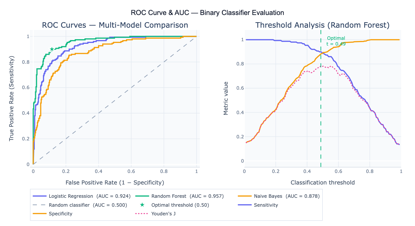
Preview
What Is a ROC Curve?
The Receiver Operating Characteristic (ROC) curve is a graphical plot of a binary classifier's performance across all possible classification thresholds. It plots the True Positive Rate (TPR = sensitivity = recall) on the y-axis against the False Positive Rate (FPR = 1 − specificity) on the x-axis as the threshold varies from 1 (predict everything negative) to 0 (predict everything positive). Each point on the curve represents a (FPR, TPR) pair at a specific threshold. A perfect classifier passes through the top-left corner (FPR = 0, TPR = 1); a random classifier follows the diagonal from (0, 0) to (1, 1). The ROC curve is threshold-independent, making it a principled way to compare the discriminative ability of classifiers without committing to a specific operating point.
The Area Under the ROC Curve (AUC), also written AUROC, summarizes the entire curve as a single number between 0 and 1. Probabilistic interpretation: AUC is the probability that the classifier ranks a randomly chosen positive instance higher than a randomly chosen negative instance (the Wilcoxon-Mann-Whitney statistic). AUC = 0.5 means the classifier performs no better than chance; AUC = 0.70–0.80 is acceptable; 0.80–0.90 is excellent; > 0.90 is outstanding. AUC is robust to class imbalance — unlike accuracy, it does not change if you have 10× more negatives than positives — making it the preferred metric for imbalanced classification problems in medicine, fraud detection, and churn prediction.
The optimal threshold is the classification probability cutoff that best balances sensitivity and specificity for your specific application. Common methods: Youden's J (maximizes sensitivity + specificity − 1, geometric optimum on the ROC curve); minimum distance to corner (closest point to the ideal top-left corner); cost-based optimization (minimizes misclassification cost when false positives and false negatives have different costs). A concrete example: a disease screening test with AUC = 0.88 might use a low threshold (high sensitivity) to minimize missed cases, accepting more false positives; a confirmatory diagnostic test with the same AUC might use a higher threshold (high specificity) to minimize unnecessary treatment.
How It Works
- Upload your data — provide a CSV or Excel file with a true label column (0/1 or binary categorical) and one or more predicted probability or score columns (one per model to compare). One row per observation.
- Describe the analysis — e.g. "plot ROC curve for the 'predicted_prob' column vs 'diagnosis'; calculate AUC with 95% DeLong CI; find optimal threshold by Youden's J; compare to a second model in 'rf_prob'"
- Get full results — the AI writes Python code using scikit-learn roc_curve, scipy.stats, and Plotly to plot ROC curves, compute AUC with confidence intervals, identify the optimal threshold, and generate a sensitivity/specificity vs threshold plot
Required Data Format
| Column | Description | Example |
|---|---|---|
label | True binary outcome | 1 (positive), 0 (negative) or 'disease', 'healthy' |
score | Predicted probability or continuous score | 0.82, 0.34, 0.91 (probabilities in 0, 1) |
score_2 | Optional: second model's scores for comparison | 0.75, 0.41, 0.88 |
Any column names work — describe them in your prompt. Predicted probabilities must be for the positive class. If your model outputs scores on any scale (not 0,1), the ROC curve is still valid — the ranking is all that matters.
Interpreting the Results
| Output | What it means |
|---|---|
| AUC | Area under ROC curve — probability of correctly ranking a random positive above a random negative |
| 95% CI on AUC | DeLong method confidence interval — if CI excludes 0.5, classifier is significantly better than random |
| Sensitivity (TPR) | True positive rate at the chosen threshold — fraction of positives correctly identified |
| Specificity | True negative rate at the chosen threshold = 1 − FPR |
| Youden's J index | Sensitivity + Specificity − 1 at each threshold — maximized at the optimal operating point |
| Optimal threshold | Score cutoff that maximizes Youden's J (or minimizes distance to top-left corner) |
| PPV / NPV | Positive / negative predictive value at the chosen threshold — depend on class prevalence |
| DeLong test | Compares AUC of two classifiers; p-value < 0.05 means one discriminates significantly better |
| Partial AUC | AUC restricted to a FPR range (e.g. 0–0.1) — relevant when only high-specificity operating points matter |
Example Prompts
| Scenario | What to type |
|---|---|
| Basic ROC + AUC | plot ROC curve for predicted probabilities vs true labels; calculate AUC with 95% CI; annotate AUC on plot |
| Optimal threshold | ROC curve; find optimal threshold by Youden's J; report sensitivity, specificity, PPV, NPV at that threshold |
| Multi-model comparison | compare ROC curves for logistic_prob and rf_prob; DeLong test for AUC difference; which model is significantly better? |
| Threshold plot | plot sensitivity, specificity, and Youden's J vs threshold; mark the optimal operating point |
| Class imbalance | ROC curve for imbalanced dataset (5% positive rate); also plot precision-recall curve; compare AUC and AUPRC |
| Partial AUC | compute partial AUC for FPR 0–0.1 (high specificity region); standardize to [0,1] scale |
| Cross-validated AUC | 5-fold cross-validated ROC curve with mean ± SD band; report mean AUC and 95% CI |
| Cost-sensitive threshold | find threshold that minimizes total cost assuming false negative costs 5× more than false positive |
Assumptions to Check
- Binary outcome — ROC curves apply to binary classifiers (positive/negative, disease/healthy, fraud/legitimate); for multi-class problems, compute one-vs-rest ROC curves for each class
- Calibrated probabilities — the ROC curve only requires correct ranking (not calibrated probabilities), so raw scores, log-odds, or decision function values all work; however, threshold interpretation requires well-calibrated probabilities — check with a calibration plot
- Independent test set — computing AUC on training data inflates the estimate; use a held-out test set, k-fold cross-validation, or bootstrap resampling
- Sufficient positives — AUC is unreliable with very few positives (< 20–30); the CI will be wide and the optimal threshold estimate noisy
- Class prevalence affects PPV/NPV — sensitivity and specificity are prevalence-independent but PPV and NPV depend heavily on the positive rate in your population; a 95% sensitivity test with 1% disease prevalence has PPV ≈ 16% (most positives are false positives)
Related Tools
Use the Logistic Regression calculator to build a logistic regression model and generate the predicted probabilities needed for ROC analysis. Use the Chi-Square Test Calculator to evaluate a classifier at a fixed threshold using a 2×2 confusion matrix. Use the Power Analysis Calculator to determine the sample size needed for a study aiming to achieve a specified AUC. Use the Volcano Plot Generator for visualizing feature importance scores from a classifier alongside significance.
Frequently Asked Questions
When should I use AUC vs accuracy?Accuracy (fraction of correct predictions) is appropriate only when classes are balanced and false positives and false negatives have equal cost. In most real-world problems — disease diagnosis, fraud detection, churn prediction — the positive class is rare (class imbalance) and the two error types have very different costs. A classifier that predicts "negative" for all samples achieves 99% accuracy on a 1% positive-rate dataset while being completely useless. AUC is unaffected by class imbalance because it evaluates ranking performance across all thresholds. Use AUC for model selection and comparison; report sensitivity, specificity, PPV, and NPV at your chosen operating threshold for clinical or operational use.
What is the DeLong method for comparing two AUC values? The DeLong test (DeLong et al., 1988) computes the variance and covariance of two AUC estimates from the same test set, accounting for the fact that the same subjects were scored by both classifiers. It then produces a z-statistic and p-value for the hypothesis AUC₁ = AUC₂. Because the same subjects appear in both curves, a paired test is more powerful than independent comparison. The test is asymptotically normal and works well for n ≥ 30. A significant DeLong p-value (< 0.05) means one model discriminates significantly better; a non-significant result means the data cannot distinguish the two models' performance (not that they are identical). Ask the AI to "compare AUC for logistic_prob and rf_prob using DeLong test; report Z-statistic, p-value, and 95% CI on the AUC difference".
What is the difference between ROC-AUC and Precision-Recall AUC? The ROC curve measures the trade-off between true positive rate and false positive rate — it is symmetric with respect to class balance and stable when the negative class is large. The precision-recall (PR) curve measures the trade-off between precision (PPV) and recall (sensitivity) — it is highly sensitive to class imbalance and collapses to a near-zero baseline when positives are rare. For highly imbalanced datasets (< 5% positives), the PR curve and its area (AUPRC) are more informative than ROC-AUC because they directly reflect the practical precision achieved at a given recall level. For balanced datasets, the two measures tend to agree on relative model rankings. Best practice: report both AUC and AUPRC for imbalanced classification problems.
Why do I get different AUC values from different tools? AUC can be estimated in two ways: (1) trapezoidal rule on the empirical ROC curve (scikit-learn default) — exact but may interpolate poorly when the curve has few points; (2) Wilcoxon-Mann-Whitney statistic — exact rank-based calculation giving the same result as the trapezoidal rule for large n. Differences between tools arise from: (a) whether the AUC is computed on the training set vs test set; (b) whether cross-validation is used; (c) how ties in the score are handled; (d) whether the curve is micro-averaged, macro-averaged, or per-class for multi-class problems. The largest differences come from training vs test evaluation — always specify which you're computing.