Confusion Matrix Calculator with Sensitivity and Specificity
Create confusion matrices online from Excel, CSV, or cell counts. Calculate sensitivity, specificity, PPV, NPV, F1, MCC, and kappa with AI.
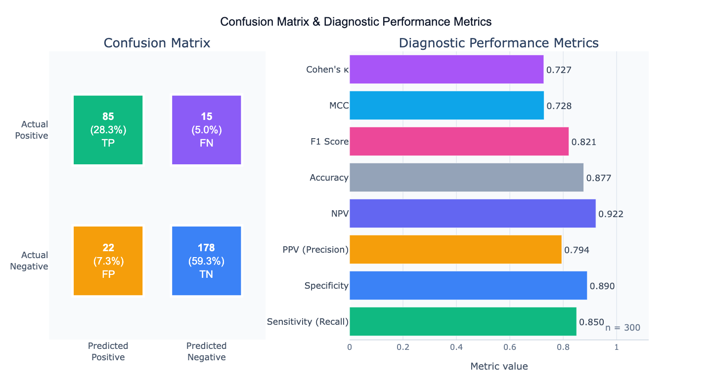
Preview
What Is a Confusion Matrix?
A confusion matrix is a table that summarizes the performance of a binary (or multi-class) classifier by cross-tabulating predicted versus actual class labels. For a binary classifier, the four cells are: True Positives (TP) — correctly predicted positives; True Negatives (TN) — correctly predicted negatives; False Positives (FP) — negatives incorrectly predicted as positive (Type I errors); and False Negatives (FN) — positives incorrectly predicted as negative (Type II errors). All other diagnostic performance metrics derive from these four numbers. The confusion matrix is the starting point for evaluating any binary classifier — a disease screening test, a fraud detection model, a quality control system, or a machine learning classifier.
From the four cells, a complete set of diagnostic performance metrics can be derived. Sensitivity (= recall = true positive rate) = TP/(TP+FN) measures how well the test finds true positives — critical for screening tests where missing a disease case is dangerous. Specificity (= true negative rate) = TN/(TN+FP) measures how well the test avoids false alarms — critical when false positives are costly (unnecessary surgery, treatment side effects). Positive Predictive Value (PPV) = TP/(TP+FP) is the probability that a positive test result is truly positive, which depends on disease prevalence. Negative Predictive Value (NPV) = TN/(TN+FN) is the probability that a negative test truly rules out the condition.
Summary metrics that balance multiple aspects: F1 score = 2 × (PPV × sensitivity) / (PPV + sensitivity) — the harmonic mean of precision and recall, appropriate when both false positives and false negatives matter. Matthews Correlation Coefficient (MCC) = (TP×TN − FP×FN) / √((TP+FP)(TP+FN)(TN+FP)(TN+FN)) — a single balanced metric particularly recommended for imbalanced datasets, ranging from −1 (perfect disagreement) to +1 (perfect prediction). Cohen's κ measures agreement corrected for chance. None of these single numbers fully replaces the full confusion matrix — always report the four cell counts alongside derived metrics.
How It Works
- Upload your data — provide a CSV or Excel file with a true label column and a predicted label column (one row per observation), or simply describe the four cell counts directly in your prompt without uploading a file.
- Describe the analysis — e.g. "confusion matrix comparing 'actual' vs 'predicted' columns; report all metrics including sensitivity, specificity, PPV, NPV, F1, MCC, and kappa; heatmap visualization"
- Get full results — the AI writes Python code using scikit-learn confusion_matrix and Plotly to produce the heatmap with annotated cell counts and percentages, and a complete metrics summary table
Required Data Format
| Column | Description | Example |
|---|---|---|
actual | True class labels | 1 (positive), 0 (negative) or 'disease', 'healthy' |
predicted | Predicted class labels | 1, 0 (same classes as actual) |
Any column names work — describe them in your prompt. For multi-class problems, provide all class labels in both columns. If you already have the 4 cell counts, describe them directly: "TP=85, FN=15, FP=22, TN=178" — no file upload needed.
Interpreting the Results
| Metric | Formula | What it means |
|---|---|---|
| Sensitivity (Recall) | TP / (TP + FN) | Fraction of true positives correctly identified — critical for screening |
| Specificity | TN / (TN + FP) | Fraction of true negatives correctly identified — critical for confirmation |
| PPV (Precision) | TP / (TP + FP) | Probability a positive result is truly positive — depends on prevalence |
| NPV | TN / (TN + FN) | Probability a negative result is truly negative |
| Accuracy | (TP + TN) / n | Overall fraction correct — misleading for imbalanced classes |
| F1 Score | 2·PPV·Sensitivity / (PPV + Sensitivity) | Harmonic mean of precision and recall — use for imbalanced data |
| MCC | (TP·TN − FP·FN) / √(...) | Balanced single metric; best for imbalanced classes; range −1, +1 |
| Cohen's κ | (p_o − p_e) / (1 − p_e) | Agreement corrected for chance; κ > 0.8 = strong agreement |
| LR+ | Sensitivity / (1 − Specificity) | Positive likelihood ratio — how much the test increases disease odds |
| LR− | (1 − Sensitivity) / Specificity | Negative likelihood ratio — how much the test decreases disease odds |
Example Prompts
| Scenario | What to type |
|---|---|
| From data columns | confusion matrix from 'actual' vs 'predicted' columns; sensitivity, specificity, PPV, NPV, F1, MCC, and kappa |
| From cell counts | confusion matrix with TP=85, FN=15, FP=22, TN=178; compute all diagnostic metrics with 95% Wilson CI |
| Multi-class | multi-class confusion matrix for 4 classes (0,1,2,3); per-class precision, recall, F1; macro and weighted averages |
| Prevalence adjustment | test sensitivity=85%, specificity=90%; compute PPV and NPV at disease prevalence of 1%, 5%, 10%, and 20% |
| Threshold comparison | confusion matrices at thresholds 0.3, 0.5, 0.7; compare sensitivity/specificity tradeoff across thresholds |
| Confidence intervals | confusion matrix TP=85, FN=15, FP=22, TN=178; 95% Wilson confidence intervals for sensitivity and specificity |
| Normalized matrix | normalized confusion matrix (row-normalized) showing recall per class; annotate with counts and percentages |
Assumptions to Check
- Binary vs multi-class — for multi-class problems, sensitivity and specificity are computed per class (one-vs-rest); report macro-averaged and weighted-averaged metrics alongside per-class values
- Prevalence dependence of PPV/NPV — PPV and NPV change with disease prevalence; a test with 90% sensitivity and 90% specificity has PPV ≈ 50% in a 1% prevalence population and PPV ≈ 91% in a 50% prevalence population; always specify the prevalence context when reporting PPV and NPV
- Class imbalance — accuracy is misleading when classes are imbalanced (a classifier that always predicts "negative" achieves 99% accuracy at 1% disease prevalence); use F1, MCC, or the ROC-AUC for imbalanced classification evaluation
- Threshold sensitivity — all confusion matrix metrics depend on the chosen classification threshold; report the threshold used and consider whether the ROC curve (threshold-free) better represents model performance
- Representative test set — the confusion matrix must be computed on a held-out test set (or cross-validated), never on training data; in-sample confusion matrices systematically overestimate performance
Related Tools
Use the ROC Curve and AUC Calculator to evaluate the classifier across all possible thresholds — the confusion matrix is a single point on the ROC curve. Use the Fisher's Exact Test Calculator to test whether the association between predicted and actual labels is statistically significant (the confusion matrix is a 2×2 contingency table). Use the Chi-Square Test Calculator for larger contingency tables (multi-class confusion matrices with many classes). Use the Power Analysis Calculator to determine sample size needed to achieve a target sensitivity and specificity with specified precision.
Frequently Asked Questions
Which metric should I use as the primary performance measure? The answer depends on what errors cost in your application. For medical screening (where missing a disease is dangerous), maximize sensitivity — you can tolerate false positives. For confirmatory diagnosis (where unnecessary treatment is harmful), maximize specificity or PPV. For balanced binary classification with equal class prevalence, F1 score is a good primary metric. For imbalanced classification (rare positives), MCC is the most informative single number — it accounts for all four cells of the confusion matrix and is not inflated by class imbalance. For overall performance evaluation, report the full confusion matrix, sensitivity, specificity, F1, and MCC together — no single number tells the whole story.
What is the Matthews Correlation Coefficient and why is it better than F1 for imbalanced data? The MCC is the correlation coefficient between the true labels and predicted labels, ranging from −1 (all predictions wrong) to +1 (perfect prediction) with 0 meaning performance no better than chance. Unlike F1 which uses only TP, FP, and FN (ignoring TN), MCC uses all four cells. For a highly imbalanced dataset where 99% of samples are negative, a classifier predicting "always negative" achieves F1 = 0 (correctly — it has zero sensitivity) but also a very high accuracy of 99%. The MCC of this trivial classifier is 0.0, correctly indicating chance-level discrimination. This makes MCC the recommended metric by several machine learning researchers (Chicco & Jurman, 2020) for imbalanced binary classification.
How do I compute confidence intervals for sensitivity and specificity? The Wilson score interval is the recommended method for proportions with small-to-moderate sample sizes: CI = (p + z²/2n ± z√(p(1−p)/n + z²/4n²)) / (1 + z²/n), where p is the proportion (sensitivity or specificity) and z = 1.96 for 95% CI. For large samples (n > 100), the normal approximation CI = p ± 1.96 × √(p(1−p)/n) is adequate. The sensitivity CI uses n = TP + FN (total positives); the specificity CI uses n = TN + FP (total negatives). Wide CIs indicate insufficient sample size for precise performance estimates — a common problem in small validation studies. Ask the AI to "compute 95% Wilson CI for sensitivity, specificity, PPV, and NPV".
Why does PPV change with disease prevalence if sensitivity and specificity are fixed? Sensitivity and specificity are intrinsic properties of the test — they describe the test's ability to detect disease and rule out disease in diseased and healthy populations respectively. They do not change with prevalence. PPV and NPV are extrinsic — they describe what a test result means for a specific patient in a specific population with a specific prior probability (prevalence). Using Bayes' theorem: PPV = (sensitivity × prevalence) / (sensitivity × prevalence + (1−specificity) × (1−prevalence)). In a population with 1% disease prevalence and a test with 90% sensitivity and 90% specificity: PPV = (0.9 × 0.01) / (0.9 × 0.01 + 0.1 × 0.99) = 0.009 / 0.108 ≈ 8.3%. Most positive tests are false positives in low-prevalence settings — an important consideration for population screening programs.