Item Analysis Calculator for Tests and Exams
Analyze exam and survey items online from Excel or CSV data. Calculate difficulty, discrimination, and weak-item flags with AI.
Or try with a sample dataset:
Preview
What Is Item Analysis?
Item analysis is the systematic evaluation of individual test or survey questions (items) to determine whether they function as intended — distinguishing high-ability from low-ability respondents, covering the intended difficulty range, and contributing to measurement reliability. Two core statistics underpin item analysis: item difficulty (p-value), the proportion of examinees who answered the item correctly (higher p = easier item), and item discrimination, which measures how well the item differentiates between high- and low-scoring respondents. Together, these indices guide decisions about which items to retain, revise, or discard from a test bank.
The point-biserial correlation (r_pb) is the standard discrimination index for binary items — it is the Pearson correlation between the binary item score (0/1) and the total test score. An item with r_pb = 0.40 means that students who answered it correctly scored substantially higher overall; an item with r_pb near zero or negative provides no useful information and may actually mislead scoring. Classical guidelines flag items with r_pb < 0.20 as poor discriminators. The upper-lower discrimination index (D) provides an intuitive alternative: compute the proportion correct in the top 27% of scorers minus the proportion in the bottom 27%; D > 0.30 is considered adequate, D < 0.20 poor. Items with p-values outside the 0.20–0.80 range (too easy or too hard) also warrant review, as they contribute little variance to the total score.
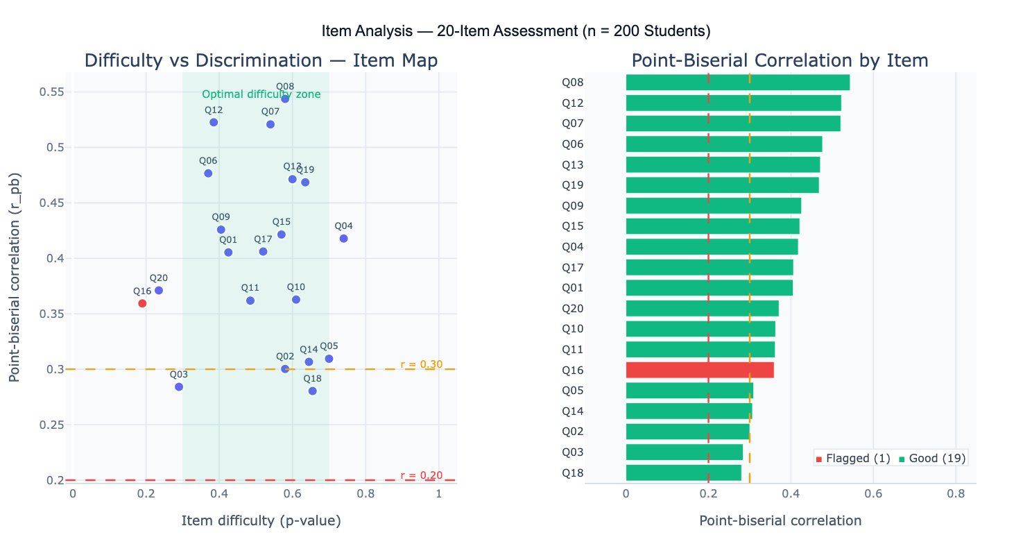
A practical example: a 30-item anatomy exam administered to 150 medical students. Item analysis reveals that item Q7 has p = 0.94 (nearly everyone answers correctly — the item is too easy, adding no discriminating information) and item Q22 has r_pb = −0.08 (students who got it right actually scored lower overall — possible keying error or ambiguous wording). Item Q15 is optimal: p = 0.52 (moderate difficulty), r_pb = 0.47 (strong discrimination). The difficulty vs discrimination scatter plot visualizes all 30 items simultaneously, with the shaded green region indicating the optimal zone (p = 0.30–0.80, r_pb ≥ 0.30).
How It Works
- Upload your data — provide a CSV or Excel file with one row per examinee and one column per item. Items should be scored 0 (incorrect/disagree) and 1 (correct/agree). A total score column is optional — the AI can compute it.
- Describe the analysis — e.g. "20 binary items, columns Q1–Q20; compute item difficulty, point-biserial r for each item; flag items with r < 0.20; difficulty vs discrimination scatter plot"
- Get full results — the AI writes Python code using pandas and Plotly to compute all item indices, flag poor-performing items, and produce the scatter plot and discrimination bar chart
Required Data Format
| Column | Description | Example |
|---|---|---|
Q1, Q2, … | Binary item score | 1 (correct) or 0 (incorrect) |
student_id | Optional: examinee identifier | S001, student_42 |
total | Optional: pre-computed total score | 18, 24 |
Any column names work — describe them in your prompt. Items must be binary (0/1). For polytomous items (0–4 Likert scale), mention that in the prompt so the AI uses the polyserial correlation instead. Missing responses should be treated as 0 (incorrect) or excluded — specify your preference.
Interpreting the Results
| Output | What it means |
|---|---|
| p-value (difficulty) | Proportion of examinees who answered correctly — 0.50 is optimal; < 0.20 or > 0.80 is problematic |
| Point-biserial r (r_pb) | Correlation between item score and total score — measures discrimination; < 0.20 is poor, ≥ 0.30 is good |
| Biserial r | Corrected version of r_pb assuming underlying continuous ability — slightly higher than r_pb |
| Discrimination index D | (% correct in top 27%) − (% correct in bottom 27%) — ≥ 0.30 is adequate, < 0.20 is poor |
| Alpha if item deleted | Cronbach's alpha of the remaining items if this item is removed — if higher than overall alpha, item is hurting reliability |
| Difficulty vs discrimination plot | Scatter of p-value vs r_pb — shaded zone shows optimal items; flagged items appear outside |
| Distractor analysis | For multiple-choice items, frequency of each answer option by performance group — distractors should attract more low scorers than high scorers |
Example Prompts
| Scenario | What to type |
|---|---|
| Basic item analysis | 20 binary items Q1–Q20; item difficulty and point-biserial r; flag r < 0.20; scatter plot; summary table |
| Alpha if deleted | item difficulty and r_pb; Cronbach's alpha if each item deleted; identify items that reduce reliability |
| Discrimination index D | upper/lower 27% discrimination index D for each item; flag D < 0.20; rank items by D |
| Distractor analysis | 5-option MCQ items; distractor frequency table for top/middle/bottom third of scorers; flag non-functioning distractors |
| Polytomous items | Likert items scored 1–5; polyserial correlation for each item; item-total correlation; flag correlations < 0.30 |
| Test revision | item analysis; identify items to discard (r < 0.20 or p > 0.85); recompute alpha after removing flagged items |
| Difficulty targeting | sort items by p-value; plot distribution of difficulty; identify how many items fall in optimal zone 0.30–0.70 |
| Item fit (IRT) | fit 1-parameter logistic (Rasch) model; item difficulty parameters; flag items with poor fit (χ² p < 0.05) |
Assumptions to Check
- Sufficient sample size — item statistics are unstable with small samples; p-values and r_pb require at least n ≥ 100 examinees for reliable estimation; with n < 50, item statistics should be interpreted cautiously and confirmed with a new administration
- Unidimensionality — item discrimination indices assume a single dominant trait underlies all items; if the test measures multiple independent constructs, run separate item analyses by subscale rather than against the total score
- Binary scoring — classical item analysis statistics (p-value, point-biserial r) apply to items scored 0/1; for partial credit or Likert items, use polyserial correlation and mean inter-item correlation instead
- Criterion-referenced vs norm-referenced — optimal difficulty depends on the test purpose: norm-referenced tests (designed to spread students out) benefit most from p ≈ 0.50; criterion-referenced mastery tests (pass/fail) may legitimately have many easy items if the material is expected to be known
- Item independence — items that scaffold on each other (if Q5 is answered wrong, Q6 is forced wrong) violate the independence assumption; verify item independence by design before interpreting discrimination indices
Related Tools
Use the Cronbach's Alpha Calculator to assess overall test reliability after completing item analysis — after removing flagged items, recompute alpha to confirm reliability improved. Use the Factor Analysis Calculator to examine the dimensional structure of the item set before running item analysis — if items load on multiple factors, item analysis should be conducted within each factor separately. Use the Cohen's Kappa Calculator when evaluating inter-rater agreement on subjectively scored items (e.g., essay questions) before computing item-level discrimination. Use the ROC Curve and AUC Calculator to evaluate item performance when the external criterion is binary (pass/fail, diagnosis/no diagnosis) — AUC for each item is equivalent to the probability that a randomly chosen passer scores higher than a randomly chosen failer on that item.
Frequently Asked Questions
What is the optimal item difficulty? For norm-referenced tests designed to rank examinees, items at p = 0.50 contribute the most variance to total scores and thus maximize the test's discriminating power. However, perfectly calibrated items at p = 0.50 are rare in practice, and the recommended range is p = 0.30–0.70 (some guidelines use 0.20–0.80). The exact optimal p depends on the number of distractors: for a 4-option MCQ where guessing probability = 0.25, the optimal p = (1 + 0.25) / 2 = 0.625, not 0.50, because random guessing raises the floor. For criterion-referenced mastery tests (e.g., licensing exams), items should be calibrated near the passing standard, and many items with p > 0.80 may be appropriate if the passing standard is high.
When should I flag an item for revision? Flag items meeting any of these criteria: (1) r_pb < 0.20 — poor discrimination; the item does not differentiate between high and low performers; (2) p > 0.90 — nearly everyone answers correctly; the item adds almost no variance; (3) p < 0.15 — nearly everyone answers incorrectly; may indicate an error in the key or unreasonably difficult content; (4) negative r_pb — examinees with higher total scores are answering the item incorrectly at higher rates; this is a red flag for a keying error, ambiguous wording, or a trick question; (5) non-functioning distractors — for MCQ items, if one or more distractors are chosen by fewer than 5% of examinees (across all ability levels), they provide no useful information and should be revised. Before revising any item, review its content alongside the statistics — sometimes a statistically poor item is pedagogically important.
What is the difference between classical test theory (CTT) and item response theory (IRT)?Classical test theory (CTT) — which underlies standard item analysis — characterizes each item by a small number of sample-dependent statistics (p-value, r_pb). These statistics depend on the ability distribution of the examinees: the same item appears harder when administered to a high-ability group. Item response theory (IRT) models the probability that a respondent with a given ability level answers correctly, producing sample-invariant item parameters (difficulty b, discrimination a, guessing c in the 3PL model). IRT is more powerful for test equating, adaptive testing, and detecting item bias (differential item functioning), but requires larger samples (n ≥ 200 for 1PL, n ≥ 500 for 2PL, n ≥ 1000 for 3PL). For routine classroom or small-scale test development, CTT item analysis is sufficient and more interpretable.
My test has very few items (5–10) — does item analysis still work? Item analysis is less stable with few items because removing or revising one item can dramatically change the total score (which is the criterion for r_pb). With 5–10 items, use the corrected item-total correlation (r_pb computed against the total score excluding the item itself — also called the "item-rest correlation") to avoid spurious inflation from the item contributing to its own criterion. The corrected r is always lower than uncorrected r, but more accurately reflects the item's independent contribution to the scale. Cronbach's alpha is also unreliable with fewer than 10 items — report the average inter-item correlation instead.