Change Point Detection Tool for Excel & CSV
Detect structural breaks online from Excel or CSV time-series data. Find regime shifts, level changes, and trend changes with AI.
Or try with a sample dataset:
Preview
What Is Change-Point Detection?
Change-point detection (also called structural break detection) identifies the moments in a time series where the underlying statistical properties shift abruptly — the mean jumps to a new level, the variance changes, the trend reverses, or the entire distributional regime switches. These transition points are called change points or breakpoints. Unlike gradual trends detected by a trendline, change points are sudden and discrete: before the break, the series behaves one way; after it, a fundamentally different pattern takes hold. Identifying these moments answers questions like "when did growth accelerate?", "when did volatility regime shift?", or "at which point did the policy intervention take effect?"
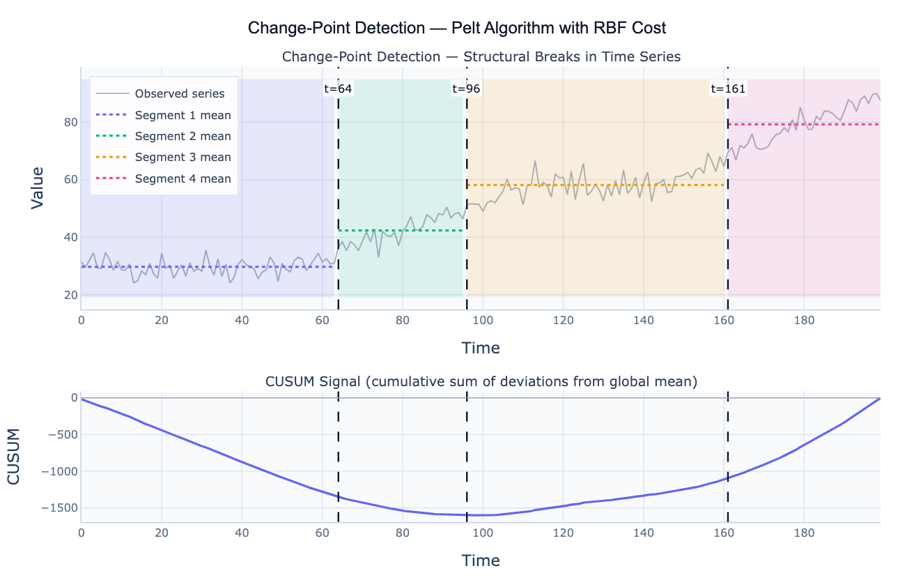
The most widely used algorithmic approach is PELT (Pruned Exact Linear Time), which finds the globally optimal set of change points by minimizing a penalized cost function. The cost function measures how well a constant-mean (or linear-trend) model fits each segment; the penalty controls how many breakpoints are allowed — a higher penalty produces fewer, more confident breakpoints, while a lower penalty finds more subtle shifts. Common cost models include L2 (optimal for mean shifts in Gaussian data), RBF (a kernel-based model that detects changes in mean, variance, and covariance simultaneously), and linear (detects changes in slope). The Bayesian Online Change-Point Detection (BOCPD) algorithm instead produces a posterior probability of a change point at each time step, allowing real-time detection as new data arrives.
The CUSUM chart (cumulative sum of deviations from the global mean) is the classical visual companion to algorithmic detection. When the process mean is stable, the CUSUM drifts near zero; when the mean shifts upward, the CUSUM rises steadily; when it shifts down, the CUSUM falls. Change points appear as inflection points or direction reversals in the CUSUM curve, making them immediately visible. A climate example: the CUSUM of global temperature anomaly shows a clear inflection around 1980, confirming the algorithmic detection of an acceleration in the warming rate at that time.
How It Works
- Upload your data — provide a CSV or Excel file with a date column and a value column. Annual, monthly, or daily data all work. One row per time point.
- Describe the analysis — e.g. "detect up to 4 change points using PELT; report breakpoint dates and segment means; CUSUM plot; annotate possible causes"
- Get full results — the AI writes Python code using ruptures for algorithmic detection and Plotly to render the segmented time series (colored regions, segment means, breakpoint lines) and the CUSUM chart
Required Data Format
| Column | Description | Example |
|---|---|---|
date | Date or time index | 1990, 2020-01, 2020-01-15 |
value | Numeric time series | 245.3, 312.1, 198.8 |
Any column names work — describe them in your prompt. For detecting breaks in a rate of change, ask the AI to compute the first difference before running detection.
Interpreting the Results
| Output | What it means |
|---|---|
| Breakpoint date/index | The time at which the structural break occurs — the last point of the preceding regime |
| Segment mean | Average value within each regime — the level before and after each break |
| Segment slope | Trend within each regime (if using linear cost) — did the growth rate change? |
| Number of breakpoints | Controlled by the penalty parameter — increase penalty for fewer (more confident) breaks |
| CUSUM inflection | Point where CUSUM changes direction — visually confirms a mean shift at that location |
| Cost / BIC | Goodness-of-fit measure for the segmented model — lower is better for a given number of breaks |
| Confidence interval | Uncertainty around the breakpoint location — wider CI = gradual or noisy transition |
| Residuals per segment | Deviation within each regime — should be white noise if the model is correctly specified |
Example Prompts
| Scenario | What to type |
|---|---|
| Mean shift detection | PELT change-point detection on annual revenue; L2 cost; report breakpoint years and segment means |
| Slope/trend break | detect changes in the growth rate (slope) of cumulative sales; use linear cost; report acceleration or deceleration at each break |
| Variance change | RBF cost change-point detection; identify periods of high and low volatility; annotate dates |
| Sensitivity sweep | run PELT with penalty 1, 5, 10, 20; plot number of breakpoints vs penalty; identify the 'elbow' where adding more breaks gives diminishing returns |
| CUSUM chart | CUSUM chart of deviations from global mean; annotate where CUSUM crosses ±2 standard deviations |
| Bayesian detection | Bayesian change-point detection; plot posterior probability of break at each time point; list top 3 most probable break dates |
Assumptions to Check
- Stationarity within segments — change-point models assume the series is stationary between breaks; seasonal effects or gradual trends within a segment will be misinterpreted as change points; deseasonalize or detrend first if needed
- Minimum segment length — most algorithms require a minimum segment size (e.g. 10–20 observations) to estimate statistics reliably; very short segments between close-together breaks are unreliable
- Penalty calibration — the penalty parameter (often BIC-based) controls the number of detected breaks; there is no universally "correct" penalty — use domain knowledge to validate whether the detected breaks correspond to real events
- Gradual vs abrupt changes — change-point methods detect abrupt transitions; a gradual drift (e.g. a slow ramp-up over 3 years) may be split into multiple artificial breakpoints; use a higher penalty or a trend-change model
- Multiple testing — examining a long series for breakpoints involves many implicit comparisons; some detected breaks may be false positives, especially at low penalty values; always validate against known events or domain knowledge
Related Tools
Use the Time Series Decomposition tool to separate trend, seasonal, and residual components before applying change-point detection to the residuals for a cleaner signal. Use the Trendline Calculator to fit separate trendlines to each identified segment after detection. Use the Seasonality Analysis tool to check whether an apparent change point is actually a shift in the seasonal pattern rather than the level. Use the Moving Median Filter to smooth the series and reduce noise before running change-point detection on slowly evolving series.
Frequently Asked Questions
How do I choose the penalty parameter? The penalty is the key tuning parameter — it trades off the goodness of fit against model complexity (number of breakpoints). Common choices: BIC-equivalent penalty = log(n) × σ² (where n is series length and σ² is noise variance), which is a reasonable default; manual elbow method (run PELT for penalty values 1 through 50, plot number of breaks vs penalty, pick the penalty at the "elbow" where adding more breaks gives little improvement); or domain knowledge (you expect approximately 2–4 breaks in a 50-year series — set the penalty to produce that number). Ask the AI to "run change-point detection for penalty values 2, 5, 10, 20, 50 and plot the number of detected breaks vs penalty".
What is the difference between PELT, Binary Segmentation, and BOCPD?PELT (Pruned Exact Linear Time) finds the globally optimal set of breakpoints in O(n) time by pruning the search space — it is the standard choice for offline analysis where all data is available. Binary Segmentation recursively splits the series at the point of greatest contrast — it is faster but suboptimal (greedy). BOCPD (Bayesian Online Change-Point Detection) computes a posterior probability of a break at each new point as data arrives — it is designed for real-time streaming use cases. For historical analysis, PELT is generally preferred; for live monitoring, BOCPD.
My algorithm finds too many or too few change points — what should I do?
If too many: increase the penalty parameter (try BIC-based penalty or double the current value); set a larger minimum segment length. If too few: decrease the penalty; check that you haven't detrended the series too aggressively (leaving no signal to detect); try a different cost function (RBF detects variance changes, not just mean shifts). You can also ask the AI to "fix the number of breakpoints at exactly 3 and find the optimal locations" — most ruptures algorithms support a fixed n_bkps parameter.
How do I validate that a detected change point is real? The strongest validation is external consistency — does the detected breakpoint date coincide with a known event? (Policy change, financial crisis, technological shift, natural disaster.) If yes, it is likely real. Statistical validation: run a Chow test (if using OLS-style segmentation) or compute the BIC for the model with the breakpoint versus the model without it — the breakpoint is justified if BIC decreases by more than 2. Ask the AI to "run a Chow test at the detected breakpoint date to test whether the structural break is statistically significant".