Survey Score Calculator for Likert Scales
Score surveys online from Excel or CSV data. Reverse-code items, compute subscales, handle missing values, and compare groups with AI.
Or try with a sample dataset:
Preview
What Is Survey Scoring?
Survey scoring is the process of converting raw item responses into meaningful composite scores — total scores, subscale scores, or standardized norms — that can be analyzed, compared across groups, and interpreted against established benchmarks. Most surveys are not analyzed at the item level; instead, items are aggregated into scales that represent latent constructs such as anxiety, job satisfaction, or quality of life. The key decisions in scoring are: which items belong to which scale (item assignment), whether any items need to be reverse-coded (flipped so that higher values consistently mean more of the construct), how to handle missing responses, and whether to express scores as raw means, sum scores, or standardized T-scores referenced to a normative population.
Reverse coding is needed for negatively-worded items — for example, in a satisfaction scale where most items ask "I enjoy my work" (1=strongly disagree, 5=strongly agree), a reverse item might ask "I often feel exhausted at work." To score this item in the same direction as the others, it is recoded so that 1→5, 2→4, 3→3, 4→2, 5→1. Failure to reverse-code negatively-worded items before summing or averaging produces artificially low subscale scores and attenuates internal consistency (Cronbach's alpha). Missing data handling — whether to exclude a respondent entirely (listwise deletion), allow prorated scores when only a few items are missing (proration), or impute missing values — significantly affects sample size and score distributions.
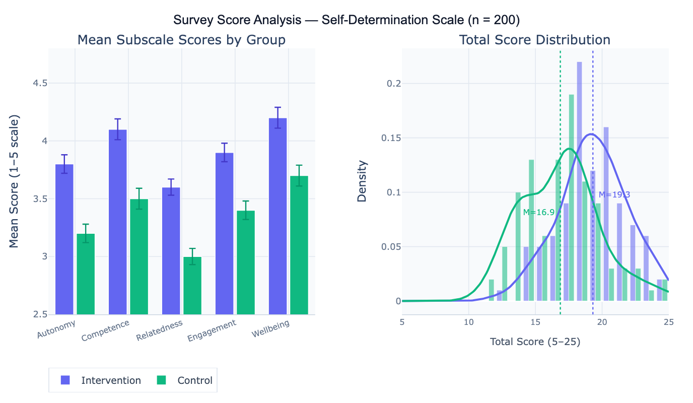
A practical example: a 20-item self-determination scale is administered to 200 students in two conditions. Items 3, 7, and 14 are negatively-worded and must be reverse-coded. After scoring, the intervention group scores significantly higher on the Autonomy subscale (M = 3.8, SD = 0.6) compared to the control group (M = 3.2, SD = 0.7), while the groups do not significantly differ on the Relatedness subscale. The total score distribution reveals that 12% of respondents score below the clinical threshold of 15/25, flagging them for follow-up.
How It Works
- Upload your data — provide a CSV or Excel file with one row per respondent and one column per survey item. Include a group or demographic column if you want group comparisons.
- Describe the scoring rules — e.g. "20 items scored 1–5; subscales: Autonomy=items 1–5, Competence=items 6–10, Relatedness=items 11–15; reverse-code items 3, 8, 12; compute total mean and subscale means; compare by group column"
- Get full results — the AI writes Python code using pandas and Plotly to reverse-code items, compute subscale and total scores, handle missing data, run descriptive statistics, and produce comparison plots
Required Data Format
| Column | Description | Example |
|---|---|---|
Q1, Q2, … | Raw item responses | 1, 2, 3, 4, 5 (Likert) |
group | Optional: grouping variable | control, intervention, male, female |
id | Optional: respondent identifier | R001, participant_12 |
Any column names work — describe them in your prompt. Items can use any numeric response scale (1–5, 0–4, 1–7, etc.). For multi-part surveys with different scales per section, describe each section's scale separately.
Interpreting the Results
| Output | What it means |
|---|---|
| Total score | Sum or mean of all items (after reverse-coding) — overall scale level |
| Subscale score | Mean or sum of items within a subscale — domain-specific score |
| Reverse-coded items | Items recoded so that higher = more of the construct throughout |
| Missing data summary | Count of missing responses per item and per respondent |
| Descriptive statistics | Mean, SD, min, max, quartiles for each scale and group |
| T-score | Standardized score with mean=50, SD=10 — allows comparison to normative samples |
| Score distribution plot | Histogram + KDE of total or subscale scores, optionally by group |
| Subscale profile plot | Bar chart of mean subscale scores with 95% CI — shows which domains differ |
Example Prompts
| Scenario | What to type |
|---|---|
| Basic total score | 10 items scored 1–5; compute total mean score; descriptive statistics; histogram |
| Reverse coding | 20-item scale; reverse-code items 3, 7, 11, 15 (1–5 scale); compute total mean; compare to non-reverse-coded version |
| Subscale scores | 4 subscales: items 1–5, 6–10, 11–15, 16–20; mean score per subscale; bar chart of subscale means with SD error bars |
| Group comparison | compute total scores; compare means between treatment and control groups; t-test; box plot by group |
| Missing data | allow prorated scores if ≤ 2 of 5 subscale items are missing; flag respondents with > 20% missing overall |
| T-score normalization | convert raw means to T-scores using normative mean=3.2, SD=0.7; how many respondents score > 1 SD below norm? |
| Percentile ranks | compute each respondent's percentile rank in the sample; flag bottom 10th percentile |
| Threshold classification | classify respondents as low/medium/high based on total score cutoffs < 30, 30–60, > 60; frequency table |
Assumptions to Check
- Item direction consistency — all items must be coded in the same direction before summing; confirm which items are negatively-worded by reviewing the questionnaire; a common error is reverse-coding an item that was already positively worded, which distorts the subscale score
- Response scale consistency — all items within a subscale should use the same response format (same number of options and same anchors); mixing a 5-point and 7-point scale within the same subscale without transformation produces non-comparable item contributions
- Missing data pattern — inspect whether missing responses are random (MAR) or concentrated in particular items or respondent groups (MNAR); listwise deletion is appropriate for ≤ 5% missing at random; for higher rates or non-random missingness, describe the imputation strategy you want
- Outlier respondents — respondents who selected the same response for every item (straight-liners) or who completed the survey in implausibly short time should be identified and potentially excluded; describe any such quality checks in your prompt
- Normative reference — if converting to T-scores or percentile ranks, the normative sample should be appropriate for your population; applying norms from a different country, age group, or clinical context can produce misleading standardized scores
Related Tools
Use the Cronbach's Alpha Calculator to assess the internal consistency reliability of each subscale after scoring — alpha should be computed on the reverse-coded items. Use the Item Analysis / Item Discrimination Calculator to evaluate whether individual items are functioning well (adequate difficulty and discrimination) before finalizing subscale composition. Use the Factor Analysis Calculator to empirically confirm that items load onto the expected subscale factors, validating the a priori subscale structure. Use the Online t-test calculator or Online ANOVA calculator to formally test whether group differences in survey scores are statistically significant. Use the Exploratory Data Analysis with AI tool for a comprehensive first look at distributions, correlations, and outliers before scoring.
Frequently Asked Questions
Should I use mean scores or sum scores? Both are mathematically equivalent for group comparisons (mean = sum / number of items), but they differ in interpretability and handling of missing data. Mean scores (average item response) are easier to interpret because they stay on the original response scale (e.g., 1–5) — a subscale mean of 3.8 out of 5 has an intuitive meaning. Sum scores are preferred when comparing against published cut-points derived from sum totals (e.g., PHQ-9 depression screening uses sum scores with specific thresholds). For missing data, mean scores naturally prorate — a respondent who skips one of five items still gets a meaningful mean from four items — while sum scores are deflated by any missing items unless imputation is applied first. Choose based on how the scale was validated and what cut-points (if any) were established.
How do I know which items to reverse-code? Reverse-coded items are specified in the questionnaire's scoring manual or user guide — do not infer them from the data alone. Common clues in the question wording: positively-framed items describe the presence of the construct ("I feel energized at work"), while reverse items describe its absence or opposite ("I feel drained at work"). A data-based check: if an item has a negative correlation with the total score (or with most other items), it is likely negatively-worded and needs reverse-coding. After reverse-coding, all items should have positive inter-item correlations. If any item still correlates negatively after reverse-coding, it may belong to a different construct or contain ambiguous wording.
What is a T-score and when should I report it? A T-score transforms raw subscale means into a standardized metric with mean = 50 and SD = 10 in a reference population. T-scores allow scores from different subscales (even those with different response scales) to be compared on the same metric, and allow an individual's score to be located relative to the normative group (T = 60 = 1 SD above the population mean). Report T-scores when: (1) a validated normative sample exists for your instrument; (2) you are comparing scores across subscales with different item counts or response scales; (3) you are screening against established clinical thresholds defined in T-score units. Do not construct T-scores using your own sample as the normative reference unless you are explicitly developing local norms — this produces T-scores that describe relative standing within your sample only, not in the broader population.
How should I handle respondents with too many missing items? The standard practice is to define a missing data threshold per subscale — commonly, allow prorated scoring if no more than 20–25% of items are missing (e.g., ≤ 1 of 5 items, or ≤ 2 of 10 items), and exclude the respondent from that subscale if more items are missing. For the total score, require a minimum number of valid subscale scores. Always report how many respondents were excluded and whether exclusion was differential across groups — if one group has substantially more missing data, this can bias comparisons. When missing data exceed 5% of the total, a brief sensitivity analysis comparing results with and without imputation adds rigor.