Linear Mixed Effects Model
Fit linear mixed effects models online from Excel or CSV data. Model clustered or longitudinal outcomes with fixed and random effects using AI.
Or try with a sample dataset:
Preview
What Is a Linear Mixed Effects Model?
A linear mixed effects model (LMM, also called a multilevel model or hierarchical linear model) extends ordinary linear regression to handle data where observations are not independent — specifically, clustered data (students within schools, patients within hospitals) and repeated measures data (multiple measurements per subject over time). The "mixed" in the name refers to the combination of fixed effects (population-level parameters estimated the same way as in ordinary regression) and random effects (subject- or group-specific deviations from the fixed effects that are modeled as draws from a probability distribution). This structure allows LMMs to correctly account for within-cluster correlation without discarding data from partially-observed subjects.
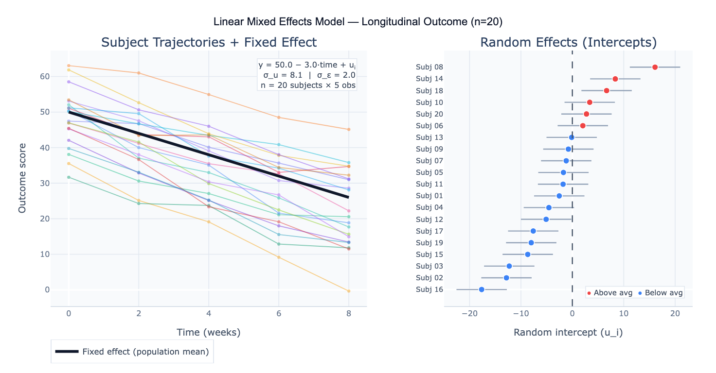
The model is written as: y = Xβ + Zu + ε, where X is the design matrix for fixed effects (β), Z is the design matrix for random effects (u ~ N(0, G)), and ε ~ N(0, R) is the residual. The most common specification is the random intercept model: each subject has their own baseline level (random intercept u_i), but the rate of change over time (the slope) is assumed the same for everyone. The random slope model additionally allows each subject to have a different rate of change, capturing heterogeneity in trajectories. Random effects are not estimated as free parameters — instead, their variance (σ²_u) is estimated, and individual-level predictions (BLUPs — Best Linear Unbiased Predictors) are shrunk toward the group mean in proportion to the reliability of each subject's data.
A concrete example: a clinical trial measures pain scores in 80 patients at baseline, 1 month, 3 months, and 6 months. Some patients miss visits, creating an unbalanced dataset that would require listwise deletion in RM-ANOVA. An LMM with random intercept per patient and fixed effects of time and treatment group correctly uses all available data, handles the missing observations under a missing-at-random (MAR) assumption, and produces: fixed effect of treatment = −12.3 points (95% CI: −18.1 to −6.5, p < 0.001); fixed effect of time = −2.1 points/month; random intercept variance σ²_u = 48.2 (ICC = 0.63, meaning 63% of total variance is between-patient). The random effects plot reveals that 6 patients have systematically higher pain throughout the study, suggesting an unmeasured subgroup.
How It Works
- Upload your data — provide a CSV or Excel file in long format: one row per observation, with columns for the outcome, grouping variable (subject/cluster ID), time or condition variable, and any predictors. Unbalanced data (different numbers of observations per subject) is fully supported.
- Describe the model — e.g. "outcome = pain_score; fixed effects = time, treatment; random intercept per patient_id; report fixed effects table with 95% CI; plot trajectories; caterpillar plot of random intercepts"
- Get full results — the AI writes Python code using statsmodels MixedLM or pymer4 to fit the model, extract fixed and random effects, compute ICC, plot individual trajectories, and produce caterpillar plots of random effects
Required Data Format
| Column | Description | Example |
|---|---|---|
subject_id | Grouping variable (cluster/subject) | P001, school_12 |
time | Within-subject variable | 0, 1, 3, 6 (months) |
outcome | Continuous response variable | 42.3, 38.1, 29.5 |
treatment | Fixed effect predictor | control, treated |
covariate | Optional: additional predictors | age, sex, baseline |
Data must be in long format (one row per observation per subject). Wide format (one column per time point) must be reshaped — ask the AI to "reshape from wide to long format first".
Interpreting the Results
| Output | What it means |
|---|---|
| Fixed effect estimate (β) | Population-average effect of each predictor — interpreted like regression coefficients |
| 95% CI on fixed effects | Uncertainty in the population-level estimate |
| t-value / p-value | Significance of each fixed effect (approximate df from Satterthwaite or Kenward-Roger method) |
| Random effect variance (σ²_u) | How much subjects differ from each other in their intercepts (or slopes) |
| Residual variance (σ²_ε) | Within-subject residual variation unexplained by the model |
| ICC (Intraclass Correlation) | σ²_u / (σ²_u + σ²_ε) — proportion of variance due to between-subject differences |
| BLUPs | Subject-specific random effect predictions — used for individual trajectory plots |
| AIC / BIC | Model fit criteria for comparing alternative model specifications (lower = better) |
| Caterpillar plot | Random effects sorted with 95% CI — subjects whose CI excludes zero are reliably above/below average |
Example Prompts
| Scenario | What to type |
|---|---|
| Random intercept model | `LMM: pain_score ~ time + treatment + (1 |
| Random slope model | `LMM with random slope: score ~ time + (1 + time |
| Interaction effect | `LMM: outcome ~ time * group + (1 |
| Clustered cross-sectional | `LMM: test_score ~ SES + school_size + (1 |
| Model comparison | fit 3 models: (1) random intercept, (2) random slope, (3) intercept + slope; compare AIC/BIC; likelihood ratio test |
| Variance components | report variance components: random intercept variance, residual variance, ICC; caterpillar plot of random intercepts |
| Missing data | LMM handles missing data; report how many observations per subject; compare to listwise deletion RM-ANOVA |
| Predictions | plot fixed effect trajectory with 95% CI band; overlay individual BLUPs for each subject |
Assumptions to Check
- Linearity — the relationship between predictors and the outcome is linear at both the within-subject and between-subject level; inspect residual plots and consider adding polynomial terms or log-transforming skewed variables if curvature is visible
- Normality of random effects — random effects are assumed ~ N(0, σ²_u); inspect with a Q-Q plot of the BLUPs; moderate deviations are acceptable with n ≥ 50 clusters; severe non-normality (bimodal or heavily skewed BLUPs) may indicate model misspecification or unmodeled subgroups
- Normality of residuals — level-1 residuals (ε) should be approximately normal; check with a Q-Q plot; LMMs are robust to moderate non-normality with large datasets
- Homoscedasticity — residual variance should be constant across fitted values and time; heteroscedasticity can be addressed by modeling a variance structure (e.g., allowing variance to differ by group or increase over time)
- Missing data mechanism — LMMs produce valid estimates under missing at random (MAR) — missingness may depend on observed variables but not on unobserved outcomes; if data are missing not at random (MNAR, e.g., patients drop out because they got worse), LMM estimates will be biased and a selection model or pattern-mixture model is needed
- Sufficient cluster size — random effects are estimated from the variance across clusters; with < 5–10 clusters, random effect variance estimates are unreliable; with > 30 clusters and ≥ 5 observations per cluster, LMM performs well
Related Tools
Use the Repeated Measures ANOVA Calculator when you have balanced data (all subjects at all time points), no covariates, and want a simpler analysis — RM-ANOVA is a special case of LMM; for missing data or unbalanced designs, LMM is preferred. Use the Multiple Regression calculator for cross-sectional data where observations are independent — LMM is needed only when observations are clustered or repeated. Use the Cox Proportional Hazards Model Calculator when the outcome is time to an event (survival analysis) rather than a continuous measurement — the frailty model (Cox with random effects) is the survival analysis analogue of LMM. Use the Residual Plot Generator to diagnose assumption violations in the LMM residuals after fitting.
Frequently Asked Questions
What is the difference between a mixed effects model and repeated measures ANOVA? Repeated measures ANOVA and LMM answer the same question but under different constraints. RM-ANOVA requires complete, balanced data (every subject measured at every time point), does not easily handle time-varying covariates, and uses an F-test based on the sphericity assumption. LMM handles unbalanced and missing data (using all available observations per subject under MAR), naturally incorporates time-varying and between-subject covariates, allows random slopes (heterogeneous rates of change), and models the correlation structure explicitly. For simple balanced designs without covariates, the two approaches give equivalent results. For anything more complex — missing data, unequal time points, subject-specific slopes, multiple random factors — LMM is the appropriate tool.
What does the ICC tell me and why does it matter? The intraclass correlation coefficient (ICC) = σ²_u / (σ²_u + σ²_ε) measures what fraction of total outcome variance is due to between-subject (between-cluster) differences. ICC = 0.63 means 63% of variance in pain scores is explained by stable patient-level characteristics — patients are remarkably consistent relative to within-patient fluctuation. High ICC (> 0.5) means individual differences dominate and modeling them is critical — ignoring clustering (using ordinary regression) would severely underestimate standard errors and produce false-positive fixed effect tests. Low ICC (< 0.05) means clustering has little impact and ordinary regression is adequate. ICC also informs sample size calculations for clustered designs: high ICC requires more clusters to achieve the same power as an unclustered design.
Should I use maximum likelihood (ML) or restricted maximum likelihood (REML)? Use REML (restricted maximum likelihood) when estimating variance components (random effect variances, ICC) and when you are not comparing models with different fixed effects — REML produces unbiased variance estimates. Use ML when comparing models with different fixed effects structures using likelihood ratio tests (LRT) — REML likelihood values are not comparable across models with different fixed effect specifications because REML integrates out the fixed effects. The practical workflow: use REML for your final model's parameter estimates and standard errors; use ML for model selection (comparing models with different fixed effects by LRT or AIC/BIC).
My model won't converge — what should I do? Convergence problems are common in complex random effects structures. Try these fixes in order: (1) Simplify the random effects — remove random slopes and start with random intercept only; (2) Scale your predictors — center continuous predictors (subtract mean) and standardize (divide by SD); unscaled predictors create numerical issues; (3) Check for multicollinearity — highly correlated predictors cause estimation instability; (4) Increase iterations — some optimizers need more iterations for complex models; (5) Try a different optimizer — switch between L-BFGS-B, Nelder-Mead, and Powell; (6) Reduce model complexity — if random slope variance is estimated near zero, remove that random slope; a near-zero random effect variance is a sign it is not needed.