Repeated Measures ANOVA Calculator
Run repeated measures ANOVA online from Excel or CSV data. Test within-subject effects, sphericity, and post-hoc differences with AI.
Or try with a sample dataset:
Preview
What Is Repeated Measures ANOVA?
Repeated measures ANOVA (also called within-subjects ANOVA) is a statistical test for comparing means across three or more conditions when the same participants are measured in each condition. Because every participant contributes data to all conditions, between-person variability can be statistically removed from the error term — this makes repeated measures ANOVA more powerful than between-subjects ANOVA (which would require different participants per condition) while requiring fewer total participants. It is the standard analysis for within-subject experimental designs, longitudinal studies with multiple time points, and crossover trials.
The core advantage of repeated measures designs is the removal of individual differences as a source of error. In a between-subjects design, person A's baseline personality, physiology, and history contribute noise to every comparison. In a repeated measures design, each person serves as their own control — the ANOVA partitions the total variance into: within-subjects variance (how scores change across conditions for each person), between-subjects variance (how people differ from each other on average, which is removed from the error), and residual error (within-subjects variance not explained by the conditions). The F-ratio = MS_within-treatment / MS_error is therefore more sensitive than its between-subjects counterpart.
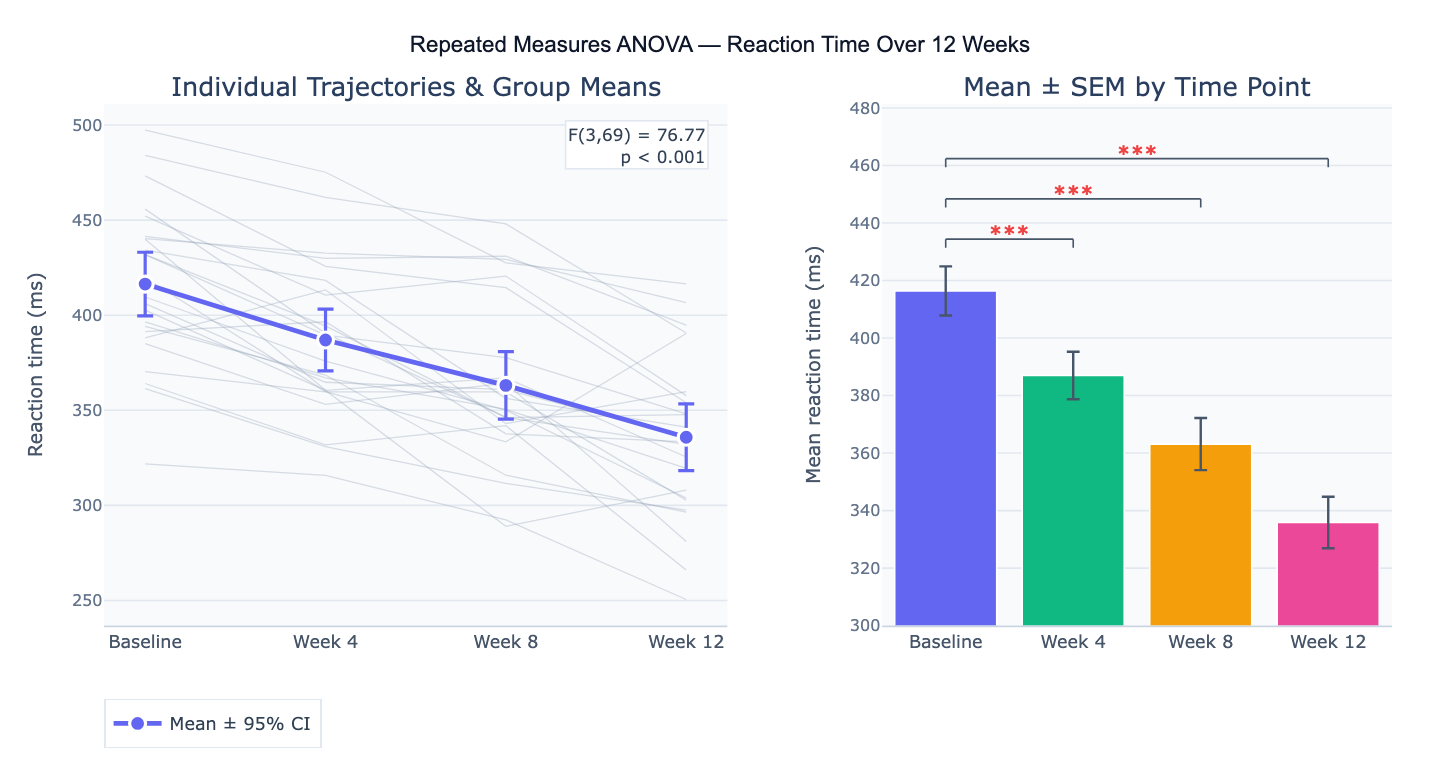
A concrete example: 20 patients complete a cognitive task at baseline and after 4, 8, and 12 weeks of training. A repeated measures ANOVA tests whether mean reaction time differs significantly across the four time points (F(3,57) = 45.2, p < 0.001, η² = 0.70). Post-hoc Bonferroni-corrected comparisons reveal that reaction time improves significantly from baseline to each subsequent time point (all p < 0.01), but the difference between week 8 and week 12 is not significant (p = 0.28), suggesting the training effect plateaus after 8 weeks. The individual trajectory plot reveals that all but 2 participants show consistent improvement, validating the group-level finding.
How It Works
- Upload your data — provide a CSV or Excel file in wide format (one row per subject, one column per condition/time point) or long format (one row per observation with subject ID, condition, and outcome columns). Describe which format you have.
- Describe the analysis — e.g. "4 time points in columns T1–T4, one row per participant; repeated measures ANOVA; Mauchly's sphericity test; Greenhouse-Geisser correction; Bonferroni post-hoc vs baseline; line plot with error bars"
- Get full results — the AI writes Python code using pingouin and Plotly to run the RM-ANOVA, Mauchly's test, apply sphericity corrections, run post-hoc pairwise tests, compute effect sizes (η², ηₚ²), and produce individual trajectory and group mean plots
Required Data Format
Wide format (preferred for simple designs):
subject | baseline | week_4 | week_8 | week_12 |
|---|---|---|---|---|
| P01 | 420 | 395 | 368 | 350 |
| P02 | 445 | 410 | 382 | 361 |
Long format (required for mixed designs):
subject | time | score |
|---|---|---|
| P01 | baseline | 420 |
| P01 | week_4 | 395 |
Any column names work — describe the format in your prompt. Missing values in any time point exclude that subject listwise from the RM-ANOVA.
Interpreting the Results
| Output | What it means |
|---|---|
| F-statistic | Ratio of between-condition variance to residual error — larger F = stronger evidence against null |
| p-value | Probability of F this large (or larger) under the null hypothesis of equal condition means |
| η² (eta-squared) | Effect size: proportion of total variance explained by the within-subject factor — 0.01 small, 0.06 medium, 0.14 large |
| ηₚ² (partial eta-squared) | Effect size excluding between-subjects variance — typically reported in repeated measures designs |
| Mauchly's W | Tests sphericity assumption — significant (p < 0.05) means sphericity is violated; correction required |
| Greenhouse-Geisser ε | Sphericity correction factor (0 < ε ≤ 1) — reduces df when sphericity is violated; smaller ε = more severe violation |
| Huynh-Feldt ε | Less conservative sphericity correction — use when Greenhouse-Geisser ε > 0.75 |
| Post-hoc p-values | Pairwise comparisons between conditions — Bonferroni or Holm adjusted for multiple comparisons |
| Individual trajectories | Spaghetti plot — reveals whether all participants respond similarly or if individual differences are large |
Example Prompts
| Scenario | What to type |
|---|---|
| Basic RM-ANOVA | repeated measures ANOVA for 4 time points; Mauchly's sphericity test; Greenhouse-Geisser correction; Bonferroni post-hoc; line plot |
| Mixed design | mixed ANOVA: within-subject factor = time (4 levels), between-subject factor = treatment group (2 levels); interaction effect; profile plot |
| Pairwise vs baseline | repeated measures ANOVA; post-hoc comparisons of each time point vs baseline only; Bonferroni correction for 3 comparisons |
| Effect size | RM-ANOVA with partial eta-squared and Cohen's d for each pairwise post-hoc comparison |
| Trend analysis | polynomial contrast analysis: test linear and quadratic trends across 5 time points; which trend component is significant? |
| Non-parametric alternative | Friedman test as non-parametric alternative to RM-ANOVA; Wilcoxon signed-rank post-hoc with Holm correction |
| Long format input | data in long format with columns subject, condition, score; repeated measures ANOVA; boxplot by condition with individual lines |
| Two within-subject factors | two-way repeated measures ANOVA: factor A = time (3 levels), factor B = task difficulty (2 levels); test main effects and interaction |
Assumptions to Check
- Sphericity — repeated measures ANOVA assumes that the variances of the differences between all pairs of conditions are equal (sphericity). Test with Mauchly's W: if p < 0.05, sphericity is violated and you must apply Greenhouse-Geisser (conservative, use when ε < 0.75) or Huynh-Feldt (less conservative, use when ε ≥ 0.75) correction to the degrees of freedom; with only 2 conditions sphericity is automatically satisfied (there is only one pair of differences)
- Normality of difference scores — RM-ANOVA assumes the differences between conditions are normally distributed (not the raw scores); test with Shapiro-Wilk on each pairwise difference; with n ≥ 30 the test is robust to non-normality by the central limit theorem; for small n with clearly non-normal differences, use the Friedman test (non-parametric alternative)
- No outliers in difference scores — extreme outliers in the within-subject differences inflate the error term and reduce power; inspect with boxplots of difference scores and consider whether outliers represent data entry errors or genuine unusual participants
- Independence of subjects — observations from different participants must be independent; this assumption is about between-person independence, not within-person — RM-ANOVA explicitly models within-person correlation; violations occur if subjects are related (e.g., sibling pairs) and should be addressed with multilevel models
- Complete data or appropriate handling of missing values — RM-ANOVA requires complete data for each subject across all conditions by default (listwise deletion); with substantial missing data, use linear mixed models which can handle missing at random (MAR) missingness without listwise deletion
Related Tools
Use the Online ANOVA calculator when participants are different people in each condition (between-subjects design) — repeated measures ANOVA is for within-subject designs where the same participants appear in all conditions. Use the Online two-way ANOVA calculator for factorial between-subjects designs; for mixed designs (one within, one between factor) the repeated measures approach handles the within-subject component. Use the Online t-test calculator (paired t-test) for the two-condition special case — a repeated measures ANOVA with exactly 2 conditions gives the same p-value as a paired t-test (F = t²). Use the Power Analysis Calculator to determine sample size needed to detect a specified effect size (η²) with desired power — repeated measures designs require fewer participants than between-subjects designs for the same power.
Frequently Asked Questions
When should I use repeated measures ANOVA instead of regular (between-subjects) ANOVA? Use repeated measures ANOVA whenever the same participants provide data in each condition — for example, measuring the same patients at baseline, 3 months, and 6 months; testing the same subjects under three different drug doses in a crossover trial; or comparing reaction times in three experimental conditions in a within-subjects psychology experiment. The key benefit is statistical power: by removing between-person variability from the error term, repeated measures ANOVA can detect smaller effects with fewer participants than between-subjects ANOVA. Use between-subjects ANOVA when different participants are in each group (separate treatment and control groups) — using repeated measures ANOVA on independent groups is incorrect.
What do I do if Mauchly's test is significant (sphericity is violated)? Apply a degrees-of-freedom correction rather than abandoning the test. The Greenhouse-Geisser correction multiplies both numerator and denominator df by ε (the sphericity estimate), producing a more conservative F-test. When ε < 0.75, use Greenhouse-Geisser; when ε ≥ 0.75, use the less conservative Huynh-Feldt correction. With only 2 df for the within-subject factor (3 conditions), the corrections have minimal impact. Alternatively, use multivariate ANOVA (MANOVA) on the repeated measures, which does not require sphericity — MANOVA is preferred when n is large relative to the number of conditions. Report both the uncorrected and corrected F-statistics, and always state which correction was applied.
What is the difference between eta-squared (η²) and partial eta-squared (ηₚ²)?Eta-squared (η²) is the proportion of total variance explained by the factor: η² = SS_factor / SS_total. It includes between-subjects variance in the denominator, making it smaller (and arguably more honest). Partial eta-squared (ηₚ²) excludes between-subjects variance: ηₚ² = SS_factor / (SS_factor + SS_error), making it larger and more comparable to effect sizes from between-subjects ANOVA. Most software (SPSS, R's ez package) reports ηₚ² by default for repeated measures designs, which is why repeated measures effect sizes often look larger than between-subjects effect sizes for equivalent phenomena. Always specify which effect size you are reporting. For benchmarks: ηₚ² ≈ 0.01 small, 0.06 medium, 0.14 large (Cohen, 1988).
Can I use repeated measures ANOVA with missing data? Standard RM-ANOVA uses listwise deletion — any participant missing data at any time point is excluded entirely, which reduces power and can introduce bias if data are not missing completely at random (MCAR). With substantial missing data (> 10–15%), consider linear mixed models (LMM) instead — LMM handles missing at random (MAR) data without case exclusion by using maximum likelihood estimation, and produces valid estimates as long as the missing data mechanism is not related to unobserved values. Ask the AI to "use a linear mixed model with random intercept for subject instead of repeated measures ANOVA to handle missing data".