Lineweaver-Burk Plot Generator
Create Lineweaver-Burk plots online from Excel or CSV data. Visualize enzyme kinetics and compare inhibition patterns with AI.
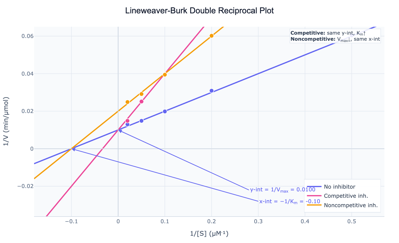
Preview
What Is a Lineweaver-Burk Plot?
A Lineweaver-Burk plot (also called a double reciprocal plot) is a linearized representation of Michaelis-Menten enzyme kinetics. By plotting 1/V on the y-axis against 1/S on the x-axis, the hyperbolic saturation curve transforms into a straight line: 1/V = (Km/Vmax) × (1/S) + 1/Vmax. The y-intercept of this line equals 1/Vmax, the x-intercept equals −1/Km, and the slope equals Km/Vmax. Before computers, this linearization allowed graphical estimation of enzyme parameters from ruler-and-graph-paper experiments — and it remains the standard diagnostic for identifying the mechanism of enzyme inhibition.
The Lineweaver-Burk plot's greatest power comes from comparing the no-inhibitor line to inhibited lines. Different inhibition mechanisms produce distinctive patterns:
- Competitive inhibition: lines intersect on the y-axis (Vmax unchanged, Km increases — same y-intercept, steeper slope)
- Noncompetitive inhibition: lines intersect on the x-axis (Km unchanged, Vmax decreases — same x-intercept, different slope and y-intercept)
- Uncompetitive inhibition: parallel lines (both Km and Vmax decrease by the same factor)
- Mixed inhibition: lines intersect in a quadrant (both Km and Vmax change independently)
These geometric patterns allow a biochemist to classify the inhibition type at a glance — one of the most common diagnostics in drug discovery and enzymology courses.
How It Works
- Upload your data — provide a CSV or Excel file with columns for substrate concentration, reaction rate, and optionally inhibitor concentration or inhibitor label. Each row is one measurement.
- Describe the analysis — e.g. "Lineweaver-Burk plot comparing no inhibitor vs 5 µM and 20 µM inhibitor; identify competitive vs noncompetitive from intersection point; extract Vmax and Km from the intercepts"
- Get full results — the AI writes Python code using numpy for linear regression on the reciprocal values and Plotly to render the double-reciprocal plot with annotated intercepts, line equations, and intersection point
Required Data Format
| Column | Description | Example |
|---|---|---|
substrate | Substrate concentration (any unit) | 1, 2, 5, 10, 50 (µM) |
rate | Initial reaction velocity | 8.2, 21.4, 54.7 (µmol/min) |
inhibitor | Optional: inhibitor concentration or label | 0, 5 µM, 20 µM |
Any column names work — describe them in the prompt.
Interpreting the Results
| Visual element | What it means |
|---|---|
| y-intercept (1/V axis) | = 1/Vmax — reads out maximum velocity |
| x-intercept (1/S axis) | = −1/Km — reads out Michaelis constant |
| Slope of line | = Km/Vmax |
| Lines intersect on y-axis | Competitive inhibition — Vmax unchanged, Km elevated |
| Lines intersect on x-axis | Noncompetitive inhibition — Km unchanged, Vmax reduced |
| Parallel lines | Uncompetitive inhibition — both Km and Vmax reduced proportionally |
| Lines intersect in upper-left quadrant | Mixed inhibition — Km and Vmax change independently |
| Curved points in reciprocal plot | Non-Michaelis-Menten kinetics — cooperativity or substrate inhibition |
Example Prompts
| Scenario | What to type |
|---|---|
| Single enzyme | Lineweaver-Burk plot, substrate column 'S_uM', rate column 'V'; annotate Vmax and Km from intercepts |
| Inhibition type | Lineweaver-Burk for no inhibitor and 10 µM compound; determine if inhibition is competitive or noncompetitive |
| Multiple inhibitor concentrations | double reciprocal plot for 0, 5, 10, 20 µM inhibitor; label each line; identify inhibition type from intersection |
| Ki estimation | Lineweaver-Burk plot, fit lines per inhibitor concentration, extract apparent Km; plot Km vs [I] to read Ki |
| Publication figure | clean Lineweaver-Burk plot, extend lines to show both intercepts, label y-intercept as 1/Vmax and x-intercept as -1/Km |
Assumptions to Check
- Initial rates only — the same requirement as Michaelis-Menten: V must be measured before significant substrate depletion
- Unweighted least-squares caveat — the double reciprocal transformation distorts error structure: points at low S (right side of plot, small 1/S) have high experimental uncertainty amplified by the 1/V transformation. Nonlinear fitting of the original V vs S data is statistically superior for parameter estimation; the Lineweaver-Burk plot is best used for visual diagnosis rather than precise parameter extraction
- Data range — points at very low S (high 1/S) dominate the line fit visually but carry the most noise; exclude extreme outliers at low substrate concentrations
- Sufficient inhibitor concentrations — identifying inhibition type requires at least 3 inhibitor concentrations spanning the Km range; a single inhibitor concentration can only tell you that inhibition is present
Related Tools
Use the Michaelis-Menten Fit for statistically optimal extraction of Vmax and Km by nonlinear least-squares fitting directly on the V vs S data. Use the Hill Equation Fit when the Lineweaver-Burk plot shows curvature — indicating cooperative kinetics. Use the Enzyme Kinetics Fit for a combined workflow that includes MM fitting, Lineweaver-Burk, and inhibition constant (Ki) estimation in one analysis.
Frequently Asked Questions
Is the Lineweaver-Burk plot the best way to estimate Vmax and Km? No — it is the best way to visualize and classify enzyme kinetics, but not the best way to estimate parameters numerically. The reciprocal transformation gives disproportionate statistical weight to low-S points (which have the most measurement noise), producing biased estimates. For precise Vmax and Km values, use the Michaelis-Menten Fit (direct nonlinear regression). Use the Lineweaver-Burk plot for quick visual diagnosis of inhibition type.
What does the x-intercept represent and how do I read it? The x-intercept of the line is −1/Km, so Km = −1 / x-intercept. For example, if the line crosses the x-axis at −0.1 (µM⁻¹), then Km = 10 µM. Note that the x-axis represents 1/S, so the left half of the plot (negative x values) corresponds to negative concentrations and is a mathematical extrapolation — the physical data all appears at positive 1/S.
How do I determine the inhibition constant Ki from a Lineweaver-Burk plot? Extract the apparent Km from the inhibited lines: for competitive inhibition, the apparent Km at inhibitor concentration I is Km(app) = Km × (1 + I/Ki). Plot Km(app) vs I — the x-intercept of that secondary plot is −Ki. Ask the AI to "extract apparent Km from each inhibitor concentration and plot Km(app) vs I to read Ki".
Why do my Lineweaver-Burk lines not converge exactly at the axis? Real data has measurement noise, so lines from different inhibitor concentrations never intersect at a perfect geometric point. Fit a linear regression to each condition's reciprocal data separately, then compute the mathematical intersection of the best-fit lines. If the intersection is near (but not exactly on) the y-axis, it is still consistent with competitive inhibition — the deviation is experimental noise, not a different mechanism.
Can I use the Lineweaver-Burk plot for non-enzyme data? Yes — any relationship that follows Michaelis-Menten-like hyperbolic saturation can be plotted in double reciprocal form: transporter kinetics (uptake rate vs. substrate for membrane transporters), receptor binding curves, or any Langmuir adsorption isotherm. The intercept and slope interpretations remain the same.