ELISA Standard Curve Calculator
Fit ELISA standard curves online from Excel or CSV data. Back-calculate concentrations, estimate LOD and LOQ, and assess precision with AI.
Preview
What Is an ELISA Standard Curve?
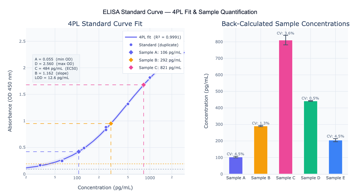
An ELISA standard curve is a calibration curve that maps the optical density (OD) measured by a plate reader to the concentration of the analyte being measured (protein, antibody, cytokine, hormone, etc.). Because ELISA signal is not linearly proportional to concentration — it saturates at high concentrations and has a non-zero background at zero analyte — the relationship follows a sigmoidal curve best described by the four-parameter logistic (4PL) model: OD = D + (A − D) / (1 + (concentration / C)^B), where A is the minimum asymptote (background OD at zero analyte), D is the maximum asymptote (plateau OD at saturation), C is the EC50 (concentration at the inflection point, midway between A and D), and B is the Hill slope (steepness). This model is the ELISA industry standard and is required by FDA and EMA guidelines for immunoassay validation.
Once the 4PL curve is fitted to the standard points, unknown sample concentrations are back-calculated by inverting the equation: concentration = C × ((A − D)/(OD − D) − 1)^(1/B). Only samples with OD values within the linear dynamic range (between approximately 20% and 80% of the OD range, or within the validated quantification range) give reliable concentrations; samples outside this range should be diluted and re-assayed. The limit of detection (LOD) is the lowest concentration distinguishable from blank with 99% confidence, typically calculated as blank mean + 3 × blank SD back-calculated to concentration. The limit of quantification (LOQ) is blank mean + 10 × blank SD — the lowest concentration that can be reliably quantified with ≤ 20% CV.
Assay quality is monitored with several acceptance criteria: R² ≥ 0.98 for the 4PL fit (lower R² indicates poor reagent quality or pipetting errors); %CV ≤ 15% between duplicate standards (≤ 20% for samples near the LOQ); accuracy of QC samples (back-calculated concentration within ±15% of nominal); and recovery of spiked samples within 80–120%. Inter-assay CV (plate-to-plate variation) is typically ≤ 20% for robust commercial ELISA kits and must be monitored across multiple runs for longitudinal studies.
How It Works
- Upload your data — provide a CSV or Excel file with a concentration column (standard concentrations in pg/mL, ng/mL, or similar), an OD column (absorbance at 450 nm or your detection wavelength), and optionally a sample column for unknown samples. Include duplicate standards on the same plate for CV calculation.
- Describe the analysis — e.g. "fit 4PL sigmoid to OD vs concentration; back-calculate samples from 'sample_od' column; report LOD, LOQ, R², and %CV for each standard level; plot standard curve with fit and unknowns annotated"
- Get full results — the AI writes Python code using scipy.optimize.curve_fit and Plotly to fit the 4PL model, back-calculate sample concentrations, compute LOD/LOQ, report %CV for replicates, and produce a log-scale standard curve plot with unknown samples annotated
Required Data Format
| Column | Description | Example |
|---|---|---|
concentration | Standard concentrations | 31.25, 62.5, 125, 250, 500, 1000, 2000 (pg/mL) |
od | Optical density reading | 0.12, 0.28, 0.55, 0.98, 1.62, 2.21, 2.48 |
replicate | Optional: duplicate/triplicate label | 1, 2 |
sample_id | Optional: unknown sample identifier | S01, S02, plasma_1 |
sample_od | Optional: OD of unknown samples | 0.42, 0.95, 1.68 |
Any column names work — describe them in your prompt. If standards and unknowns are in the same sheet, use a column to distinguish them (e.g., type = 'standard' vs 'sample'). Blank wells (zero concentration) should be included for LOD/LOQ calculation.
Interpreting the Results
| Output | What it means |
|---|---|
| 4PL parameters (A, B, C, D) | A=min OD (background), D=max OD (saturation), C=EC50 (midpoint concentration), B=Hill slope |
| R² | Goodness of fit of the 4PL model — must be ≥ 0.98 for a valid assay |
| Back-calculated concentration | Concentration of each unknown sample inverted from the 4PL curve |
| %CV (within-assay) | Coefficient of variation between duplicate/triplicate standards or samples — should be ≤ 15% |
| Accuracy (% recovery) | Back-calculated / nominal × 100% for QC standards — acceptable range 85–115% |
| LOD | Blank mean + 3 × blank SD, back-calculated to concentration — signal distinguishable from noise |
| LOQ | Blank mean + 10 × blank SD, back-calculated to concentration — reliable quantification threshold |
| Dynamic range | Concentration range between LOQ and the upper asymptote (≈ 80% of max OD) — valid measurement window |
| Residuals | Difference between observed and fitted OD at each standard — should be random within ±10% |
Example Prompts
| Scenario | What to type |
|---|---|
| Basic 4PL fit | fit 4PL sigmoid to OD vs concentration; report A, B, C, D parameters and R²; back-calculate unknown samples; log-scale plot |
| LOD and LOQ | fit 4PL standard curve; compute LOD and LOQ from blank wells (8 replicates); annotate on the curve |
| Duplicate analysis | standard curve with duplicates; compute %CV for each concentration level; flag levels where CV > 15% |
| 5PL model | fit both 4PL and 5PL models; compare R² and residuals; use 5PL if it fits significantly better |
| Plate dilution | samples were diluted 1:4 before assay; back-calculate from curve then multiply by 4 to get original concentration |
| Inter-assay CV | I have standard curves from 3 separate plates; compare EC50 (C parameter) across plates; report inter-assay CV |
| QC samples | I have 3 QC standards at low/medium/high concentration; report accuracy (% nominal) and flag if outside 85–115% |
| Full report | fit 4PL; report all parameters, R², LOD, LOQ; back-calculate all unknown samples; flag samples outside dynamic range; compute %CV for replicates |
Assumptions to Check
- Sigmoidal range coverage — the standard curve must include at least one point above and below the inflection point (EC50) to define both asymptotes; a curve that only covers the linear portion cannot reliably estimate A or D, and back-calculation will be inaccurate near the extremes
- Duplicates or triplicates — run standards in duplicate minimum; single-point standards cannot estimate within-assay precision; most regulatory and publication standards require duplicates, with some requiring triplicates for the lowest concentrations
- Sample OD within dynamic range — samples with OD < LOQ OD or OD > 90% of maximum asymptote D are outside the reliable quantification range; dilute high-OD samples and re-assay
- 4PL vs 5PL — the 5-parameter logistic (5PL) adds an asymmetry parameter; use 5PL when the curve is visibly asymmetric around the inflection point, but only with sufficient data points (≥ 8 standards) to reliably estimate all 5 parameters
- Same plate for standards and unknowns — back-calculation assumes unknowns were run on the same plate as the standards; cross-plate back-calculation introduces systematic error from plate-to-plate variation in coating, incubation, and wash conditions
Related Tools
Use the Dose-Response Curve Generator for IC50 and EC50 determination in pharmacology, which applies the same 4PL/5PL models but reports the midpoint concentration as the IC50/EC50 rather than back-calculating sample concentrations. Use the Hill Equation Fit for binding affinity and receptor occupancy curves using the Hill model. Use the Residual Plot Generator to inspect the 4PL fit residuals for systematic patterns. Use the Multiple Regression calculator to model concentration as a function of multiple predictors after back-calculating concentrations from ELISA data.
Frequently Asked Questions
Why use 4PL instead of a simple linear standard curve? ELISA signal is non-linear — at very low concentrations the OD is near background (lower asymptote A) and at very high concentrations it plateaus (upper asymptote D). If you fit a linear regression to the full concentration range, the fit will be poor and back-calculated concentrations will be systematically biased, especially at the extremes. The 4PL model correctly describes the sigmoidal shape across the entire dynamic range. Some analysts use a linear fit on the "log-linear" region (middle part of the curve) — this is less accurate but acceptable for quick estimates when samples fall confidently in the linear range. For regulatory submissions (FDA, EMA), the 4PL or 5PL model is required by bioanalytical method validation guidelines (FDA 2018, EMA 2011).
What is the difference between 4PL and 5PL? The 4PL model assumes a symmetric sigmoid — the curve rises identically on both sides of the EC50. The 5PL model adds a fifth parameter (often called F or ν — the asymmetry factor) that allows the curve to rise more steeply on one side than the other: OD = D + (A − D) / (1 + (x/C)^B)^F. When F = 1, 5PL reduces to 4PL. Use 5PL when you observe that the curve bends more sharply near the lower asymptote than the upper (or vice versa) and you have enough data points (≥ 8–10 standards) to estimate the additional parameter reliably. In practice, the 4PL is preferred for simplicity and interpretability unless the asymmetry is clearly visible in the residuals.
What do I do if my sample OD is above the standard curve maximum? If a sample OD exceeds the highest standard (or approaches D, the upper asymptote), the back-calculated concentration is unreliable because small OD changes correspond to very large concentration changes near saturation. The correct approach is to dilute the sample (e.g., 1:4 or 1:10 with assay diluent) and re-assay, then multiply the back-calculated concentration by the dilution factor. Report the original (undiluted) concentration = back-calculated × dilution factor. Never extrapolate above the standard curve range. Ask the AI to "back-calculate samples; flag any sample with OD > 90% of D as 'above range — dilute and re-assay'".
How do I calculate and report %CV? For within-assay %CV (intra-assay precision): run each standard or QC sample in duplicate or triplicate on the same plate; compute the mean and SD of the duplicate OD values or back-calculated concentrations; %CV = (SD / mean) × 100. Guidelines typically require %CV ≤ 15% for standards and samples (≤ 20% at the LOQ). For between-assay %CV (inter-assay precision): run the same QC samples across multiple plates on different days; compute %CV across the plate mean values. Report both %CV values in methods. Ask the AI to "compute %CV for each standard concentration level from duplicate ODs; flag levels > 15% in the results table".