qPCR Delta Delta Ct Calculator
Calculate Delta Delta Ct and fold change online from qPCR Ct values. Normalize to reference genes and compare conditions with AI.
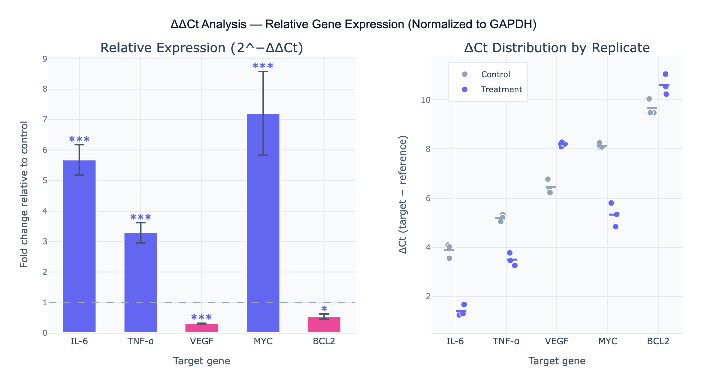
Preview
What Is the ΔΔCt Method?
The ΔΔCt method (delta delta Ct, also written 2^−ΔΔCt or Livak method) is the standard approach for relative quantification of gene expression from qPCR data. It computes the fold change in a target gene's expression between a treatment and control condition, normalized to a reference gene (housekeeping gene) to correct for differences in RNA input, reverse transcription efficiency, and loading between samples. The calculation proceeds in two steps: first compute ΔCt = Ct_target − Ct_reference for each sample (normalizing the target to the housekeeping gene); then compute ΔΔCt = ΔCt_treatment − ΔCt_control (expressing the difference relative to the control condition). The fold change is then 2^(−ΔΔCt) — a fold change of 2 means the target gene is expressed 2× higher in treatment vs control; 0.5 means 2× lower; 1 means no change.
The method assumes equal PCR efficiency between the target and reference genes — both should have efficiency within 5% of each other (ideally both near 100%). This assumption can be validated by running a standard curve for each gene and comparing slopes (see qPCR Standard Curve Calculator). If efficiencies differ by > 5%, the Pfaffl method must be used instead, which corrects for efficiency differences: Ratio = (E_target)^ΔCt_target / (E_reference)^ΔCt_reference. The choice of reference gene is also critical — an ideal reference gene has stable expression across all experimental conditions; use geNorm or NormFinder to identify the most stable reference when multiple candidates are available.
Statistical analysis of ΔΔCt data requires careful consideration: significance testing is performed on the ΔCt values (not fold changes), because ΔCt is normally distributed on the log₂ scale whereas fold changes are log-normally distributed. A two-sample t-test or one-way ANOVA on the ΔCt values produces valid p-values; performing a t-test on fold changes instead is incorrect. Error propagation — the standard error on fold change accounting for variance in both ΔCt_treatment and ΔCt_control — is done by propagating from the ΔΔCt distribution, then back-transforming to the fold-change scale as asymmetric error bars.
How It Works
- Upload your data — provide a CSV or Excel file with sample names, condition labels, Ct values for the reference gene, and Ct values for one or more target genes. One row per sample (or per technical replicate).
- Describe the analysis — e.g. "reference gene GAPDH, control condition 'untreated'; compute ΔCt for each sample, ΔΔCt relative to untreated mean, fold change = 2^(−ΔΔCt); bar chart with SEM error bars and t-test significance stars"
- Get full results — the AI writes Python code using pandas and scipy.stats to normalize Ct values, compute ΔCt and ΔΔCt, propagate errors, run statistical tests, and generate bar charts with error bars and significance annotations using Plotly
Required Data Format
| Column | Description | Example |
|---|---|---|
sample | Sample identifier | S1, S2, mouse_01 |
condition | Experimental group | control, treated, untreated |
replicate | Optional: biological replicate number | 1, 2, 3 |
GAPDH | Reference gene Ct value | 18.2, 17.9, 18.5 |
IL6 | Target gene Ct value | 24.3, 22.1, 25.0 |
ACTB | Additional target gene (optional) | 21.4, 20.8, 21.9 |
Any column names work — describe them in your prompt. Technical replicates should be averaged before ΔCt calculation, or the AI can average them automatically. Undetermined (non-amplified) Ct values should be marked as NA or the instrument's maximum cycle number.
Interpreting the Results
| Output | What it means |
|---|---|
| ΔCt | Ct_target − Ct_reference; normalizes target to housekeeping gene; lower ΔCt = higher relative expression |
| ΔΔCt | ΔCt_sample − mean(ΔCt_control); calibrates relative to control condition |
| Fold change (2^−ΔΔCt) | Expression relative to control; > 1 = upregulated, < 1 = downregulated, 1 = no change |
| SEM on fold change | Propagated from ΔCt variance; asymmetric error bars in fold-change space |
| p-value (t-test on ΔCt) | Significance of expression difference between conditions (performed on ΔCt, not fold change) |
| 95% CI on fold change | Back-transformed from ΔΔCt ± 1.96 × SEM(ΔΔCt) to fold-change scale |
| Pfaffl ratio | Efficiency-corrected fold change when target and reference efficiencies differ by > 5% |
| Reference gene stability | CV of reference gene ΔCt across samples — should be < 0.5 Ct to confirm stable expression |
Example Prompts
| Scenario | What to type |
|---|---|
| Basic ΔΔCt | reference gene GAPDH, control = 'vehicle'; compute ΔΔCt and fold change for IL-6 and TNF-α; bar chart with SEM; t-test stars |
| Multiple reference genes | normalize using geometric mean of GAPDH and ACTB Ct; compute ΔCt, ΔΔCt, and fold change; compare to single-reference normalization |
| Multiple conditions | 3 conditions: vehicle, low-dose, high-dose; reference GAPDH; ANOVA on ΔCt with Tukey post-hoc; bar chart with significance brackets |
| Pfaffl method | target efficiency 95%, reference efficiency 100%; compute Pfaffl ratio instead of 2^−ΔΔCt; compare both methods |
| Technical replicate averaging | 3 technical replicates per sample; average Ct, exclude replicates with SD > 0.5 Ct; then ΔΔCt on biological replicates |
| Log2 fold change | compute log2 fold change (= −ΔΔCt) for volcano plot input; report mean, SEM, and p-value for each gene |
| Reference gene validation | plot Ct CV for GAPDH, ACTB, and RPL13A across all samples; which reference gene is most stable? |
| Time course | 4 time points (0h, 6h, 24h, 48h); ΔΔCt relative to 0h; line chart of fold change over time with error bars |
Assumptions to Check
- Equal PCR efficiency — run a standard curve for both target and reference genes; if slopes differ by > 0.2 (efficiency difference > 5%), use the Pfaffl correction instead of the standard 2^−ΔΔCt formula
- Stable reference gene — verify that the reference gene Ct does not vary significantly across conditions (CV < 0.5 Ct); a reference gene that changes with treatment will distort all fold-change estimates; run geNorm analysis when multiple reference candidates are available
- Normal distribution of ΔCt — t-test and ANOVA on ΔCt assume normality; check with a Q-Q plot on ΔCt values; with 3 biological replicates this is hard to verify — use consistent experimental conditions to minimize variance
- No amplification in no-template control (NTC) — NTC wells must show no Ct signal (or Ct > 38); any amplification in NTC indicates contamination and invalidates the data
- Biological vs technical replicates — statistical tests require biological replicates (independently processed samples), not just technical replicates (repeated measurements of the same cDNA); t-test with only technical replicates underestimates the true variance
Related Tools
Use the qPCR Standard Curve Calculator to validate PCR efficiency for both target and reference genes before applying the ΔΔCt method — if efficiencies differ by > 5%, you must use the Pfaffl method. Use the Melt Curve Analysis tool to verify primer specificity and confirm single-product amplification before analyzing Ct values. Use the Volcano Plot Generator to visualize log2 fold change vs −log10(p-value) across many genes from a ΔΔCt experiment. Use the Online t-test calculator to run the statistical test on ΔCt values with full output if you already have the ΔCt calculated.
Frequently Asked Questions
Should I perform statistics on ΔCt or fold change? Always perform statistics on ΔCt values, not fold changes. ΔCt is approximately normally distributed (being a difference of two normally distributed Ct measurements), so t-tests and ANOVAs are valid on ΔCt. Fold change = 2^(−ΔΔCt) is log-normally distributed — applying a t-test to fold changes directly violates the normality assumption. The standard workflow is: (1) test normality of ΔCt with a Shapiro-Wilk test; (2) run a two-sample t-test on ΔCt for two groups (or one-way ANOVA for > 2 groups); (3) report the fold change with its propagated error bars as a visual summary. The p-value comes from the ΔCt test.
What is the difference between ΔΔCt and the Pfaffl method? The ΔΔCt (Livak) method assumes both the target and reference genes amplify with exactly 100% efficiency (doubling per cycle). The formula is: ratio = 2^(−ΔΔCt). The Pfaffl method relaxes this assumption by using the actual efficiency of each gene: ratio = (E_target)^ΔCt_target / (E_reference)^ΔCt_reference. If you have validated standard curves showing the target efficiency is 98% and the reference is 100%, Pfaffl gives a more accurate ratio. In practice, when both efficiencies are in the 90–110% range and within 5% of each other, the two methods give nearly identical results. Only use Pfaffl when there is a meaningful efficiency difference, as it requires additional standard curve data.
How many biological replicates do I need? A minimum of 3 biological replicates is required for any statistical test — this is a MIQE (Minimum Information for Publication of Quantitative Real-Time PCR Experiments) guideline. Three replicates allow a t-test but with low power: if the true fold change is 2× (ΔΔCt = 1) with typical ΔCt SD of 0.3–0.5, you need 4–6 biological replicates to achieve 80% power. The common error of using technical replicates (repeated measurements of the same cDNA sample) as if they were biological replicates inflates the degrees of freedom and produces falsely narrow confidence intervals. Technical replicates should be averaged first; biological replicates provide the correct error estimate.
My Ct values are undetermined (no amplification) in some samples — what do I do? Undetermined Ct values (the instrument reports 40 or "undetermined" when no amplification is detected within the cycle limit) require careful handling. Options: (1) Exclude the undetermined sample with documentation if there is a technical reason (failed reaction, degraded RNA); (2) Set to the maximum cycle number (e.g., 40) to treat it as a very low but present expression — conservative but allows arithmetic; (3) Report as "not expressed" and exclude from fold change calculation, noting the gene as below detection in that condition; (4) For statistical analysis, use a censored data approach if many samples have undetermined values. Never impute undetermined with an arbitrary value. Ask the AI to "handle undetermined Ct values: if > 1/3 of replicates are undetermined, report gene as not detected; otherwise use Ct = 40".