Boxen Plot Generator for Excel & CSV
Create boxen plots online from Excel and CSV data. Reveal tail behavior and compare large distributions with more detail than box plots.
Or try with a sample dataset:
Preview
What Is a Boxen Plot?
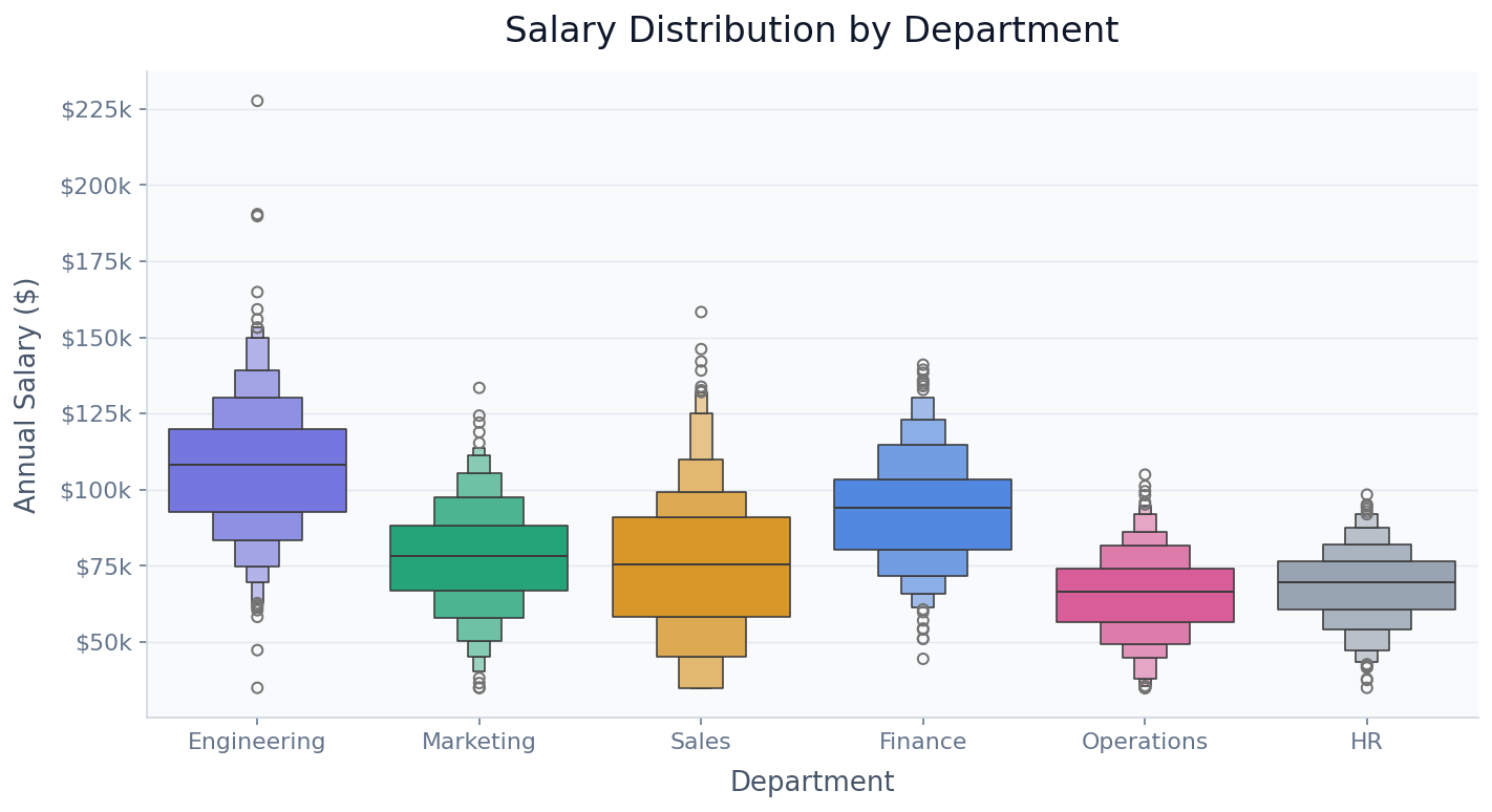
A boxen plot (formally called a letter-value plot) is an enhanced version of the box plot that reveals the full shape of a distribution by drawing multiple nested boxes, each representing a successively deeper pair of quantile levels. The central box shows the interquartile range (25th–75th percentiles), the next box out shows the 12.5th–87.5th percentile range, the next shows the 6.25th–93.75th, and so on — each level halving the remaining tail. The nesting continues until the remaining data in each tail is small enough to label as individual outlier points. This creates the distinctive "letter-value" staircase that gives the chart its formal name.
The key advantage over a standard box plot is that boxen plots show where the tails of the distribution actually are, not just a fixed whisker length. A box plot's whiskers extend to 1.5× the IQR by default, which can obscure whether a distribution has a gentle taper or an abrupt cliff. The boxen plot makes this visible: a long chain of narrow boxes means the distribution has a heavy tail; boxes that quickly shrink to individual points mean it drops off sharply. This matters in practice — salary distributions almost always have a right-heavy tail (a few very high earners), and a boxen plot shows exactly how heavy that tail is across different departments or companies.
Boxen plots outperform violin plots for large datasets (thousands of rows per group) where the kernel density estimate can be noisy or misleading at the tails, and they work better than standard box plots when you care about the distribution shape beyond the median and IQR. They are especially popular in data science and economics for comparing distributions across many groups when the tails carry meaningful information.
How It Works
- Upload your data — provide a CSV or Excel file with at least one numeric column (the variable to distribute) and one categorical column (the grouping variable). Long format works best: one row per observation.
- Describe the plot — e.g. "boxen plot of salary by department, sort by median, color each department differently"
- Get the visualization — the AI writes Python code using seaborn and matplotlib to build the nested letter-value chart
Interpreting the Results
| Visual element | What it means |
|---|---|
| Central (widest) box | Interquartile range — middle 50% of the data |
| Next box out | 12.5th–87.5th percentile — middle 75% of the data |
| Each successive box | Adds the next letter-value level, halving the remaining tail |
| Final small boxes | Near the extreme tails — only a small fraction of data lies here |
| Individual points beyond boxes | Outliers — observations beyond the last letter-value level |
| Box width at each level | Constant within a group — the nesting is in height, not width |
| Long chain of small boxes | Heavy tail — many observations far from the median |
| Few levels before points | Light tail — distribution drops off quickly past the IQR |
Example Prompts
| Scenario | What to type |
|---|---|
| Salary analysis | boxen plot of salary by job level, sort by median, color by level |
| Financial returns | boxen plot of annual stock returns by sector, log scale, highlight outliers |
| Health data | boxen plot of BMI by age group, show all quantile levels, label medians |
| Survey scores | boxen plot of customer satisfaction score by product line, sorted by median |
| Scientific data | boxen plot of gene expression by tissue type, top 8 tissues by variance |
Related Tools
Use the AI Box Plot Generator when you have fewer than ~200 observations per group — box plots are cleaner at small sample sizes where the extra quantile levels in a boxen plot would be noisy. Use the AI Violin Plot Generator when you want to see the continuous density shape rather than discrete quantile boxes — violins are more intuitive for audiences unfamiliar with letter-value plots. Use the Ridgeline Plot Generator when you have many groups ordered along a natural dimension (e.g. years, decades) and want to emphasize the shift in distribution shape across the sequence.
Frequently Asked Questions
How is a boxen plot different from a box plot? A standard box plot shows five summary statistics: minimum, Q1, median, Q3, and maximum (plus outlier points beyond 1.5× IQR). A boxen plot extends this by computing letter values — successive quantile pairs that each cover half the remaining data in the tails. For a dataset of 1,000 observations you might see 6–8 nested levels before hitting individual outlier points, revealing the full tail structure that a box plot's single whisker hides.
How many observations do I need for a boxen plot to be useful? The rule of thumb is at least 200 observations per group. With fewer observations, the outer letter-value levels are estimated from very few data points and become unreliable. For small groups (< 50 observations), a standard box plot or strip plot is more honest. Ask the AI to only draw boxen plots for groups meeting a minimum sample size threshold and use a simpler chart for small groups.
Can I control how many quantile levels are shown? Yes — ask for "show 4 letter-value levels" or "show only the IQR and the next two levels". You can also ask for "show all levels down to k=5 observations" to control how aggressively the boxes extend into the tails.
My data has a strong right skew — should I use a log scale? Yes, for highly skewed data (like salaries, revenues, or populations), ask for a "log scale on the y-axis". This spreads out the lower part of the distribution and compresses the long upper tail, making the nested boxes more legible across all groups simultaneously.
Can I overlay individual data points on top of the boxes? Yes — ask for "strip plot overlay" or "show individual points as a jitter plot on top of the boxen plot". This combines the quantile summary of the boxen plot with the raw data transparency of a strip chart, which is particularly useful when sample sizes differ across groups.