Bland-Altman Plot Generator
Create Bland-Altman plots online from Excel or CSV data. Compare measurement methods, estimate bias, and inspect limits of agreement with AI.
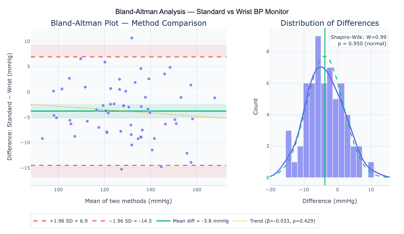
Preview
What Is a Bland-Altman Plot?
The Bland-Altman plot (also called a mean-difference plot or Tukey mean-difference plot) is the standard method for assessing agreement between two measurement methods applied to the same subjects. Introduced by Bland and Altman in 1986 in one of the most cited statistical papers in medicine, it plots the difference between the two methods (Method A − Method B) on the y-axis against the mean of the two methods ((A + B) / 2) on the x-axis for each subject. The horizontal lines show the mean difference (bias) — how much one method systematically over- or under-reads relative to the other — and the 95% limits of agreement (LoA = bias ± 1.96 × SD) — the range within which 95% of differences between the two methods are expected to fall. If the limits of agreement are clinically acceptable (narrow enough for the intended purpose), the two methods can be considered interchangeable.
The Bland-Altman method answers a question that correlation cannot: two methods can have near-perfect correlation (r ≈ 1) while one systematically reads 20 mmHg higher than the other — the correlation measures linear association, not agreement. Similarly, a paired t-test only tests whether the mean difference is zero, not whether individual measurements agree closely enough for clinical use. The Bland-Altman plot reveals all three key issues at once: systematic bias (mean difference ≠ 0), proportional bias (the difference grows larger as the mean increases, visible as a sloped scatter pattern), and heteroscedasticity (variance of differences increases with the mean).
A concrete example: comparing a new portable pulse oximeter against a hospital arterial blood gas analyzer for oxygen saturation in 60 patients. A Bland-Altman plot might show mean bias = −0.5% (portable slightly lower), LoA = −3.8% to +2.8%, and no proportional bias. If the clinically acceptable difference is ±4%, the limits of agreement fall within this range and the devices can be considered interchangeable for routine monitoring. The 95% confidence intervals on the bias and LoA quantify the uncertainty in these estimates due to finite sample size.
How It Works
- Upload your data — provide a CSV or Excel file with one column per measurement method and one row per subject. Both methods must measure the same quantity on the same subject at the same time.
- Describe the analysis — e.g. "Bland-Altman plot comparing 'standard_bp' and 'wrist_bp'; compute mean bias, LoA, 95% CI on LoA; test for proportional bias; flag outliers"
- Get full results — the AI writes Python code using scipy.stats and Plotly to compute the bias, SD, limits of agreement with CI, regression test for proportional bias, Shapiro-Wilk normality test on differences, and produce the Bland-Altman plot with all reference lines and CI bands
Required Data Format
| Column | Description | Example |
|---|---|---|
method_a | First method measurements | 118.2, 145.0, 132.5 (mmHg) |
method_b | Second method measurements | 121.4, 141.8, 135.0 (mmHg) |
subject_id | Optional: subject identifier | P001, P002 |
Any column names work — describe them in your prompt. Both columns must contain measurements on the same scale and the same subjects in the same row order. Missing values in either column will exclude that subject from the analysis.
Interpreting the Results
| Output | What it means |
|---|---|
| Mean difference (bias) | Systematic offset between methods — if close to zero, no systematic bias |
| SD of differences | Spread of individual differences — smaller SD = better agreement |
| Limits of Agreement (LoA) | bias ± 1.96 × SD — range containing ~95% of all pairwise differences |
| 95% CI on bias | Precision of the mean difference estimate — depends on sample size |
| 95% CI on LoA | Precision of the LoA bounds — widens with smaller n or larger SD |
| Proportional bias (slope) | Regression of difference on mean — significant slope = bias depends on measurement magnitude |
| % outside LoA | Fraction of points beyond the limits — should be ~5% if differences are normally distributed |
| Shapiro-Wilk test | Tests normality of differences — LoA interpretation assumes normality |
| Repeatability coefficient | 1.96 × √2 × within-subject SD — smallest detectable difference within one method |
Example Prompts
| Scenario | What to type |
|---|---|
| Basic comparison | Bland-Altman plot comparing method_a and method_b; report bias, SD, LoA, and 95% CI |
| Clinical acceptability | Bland-Altman plot; acceptable difference is ±5 mmHg; do the LoA fall within ±5? report conclusion |
| Proportional bias | Bland-Altman plot; regress difference on mean; test if slope is significantly different from zero (p < 0.05) |
| Log transformation | Bland-Altman plot on log-transformed values; ratio LoA; express bias as % (geometric mean ratio) |
| Repeated measures | Bland-Altman with 3 replicates per subject per method; use within-subject SD; adjusted LoA for repeated measures design |
| Multiple methods | Bland-Altman plots comparing Method A vs B, A vs C, and B vs C; 3 panels side by side |
| Regression-based LoA | proportional bias present; compute regression-based LoA (Bland-Altman 1999 extension) accounting for non-constant bias |
Assumptions to Check
- Normal distribution of differences — the limits of agreement assume differences are approximately normally distributed; check with a Shapiro-Wilk test on the differences and a histogram; for non-normal distributions, use a log transformation (if differences are proportional) or report percentile-based LoA
- No proportional bias — the standard Bland-Altman method assumes the bias is constant across the measurement range; if a regression of difference on mean is significant (p < 0.05), use the regression-based LoA extension (Bland & Altman, 1999) or report separate bias estimates for low, medium, and high measurement ranges
- Independent subjects — each subject should contribute one pair of measurements; if subjects are measured multiple times, use the repeated measures extension of Bland-Altman to account for within-subject correlation (otherwise LoA will be too narrow)
- Sufficient sample size — n ≥ 30–40 subjects is typically recommended for reliable LoA estimates; with n = 100+, the CI on the LoA becomes narrow enough for regulatory submissions (FDA 510(k), ISO 81060 for blood pressure devices)
- Same units and scale — both methods must be on the same measurement scale; if one uses different units, convert before analysis
Related Tools
Use the Correlation Matrix Calculator or Linear Regression to compute Pearson's r between two methods — but remember that high correlation does not imply good agreement. Use the Online t-test calculator to test whether the mean difference is significantly different from zero (paired t-test), complementing the Bland-Altman visual assessment. Use the Residual Plot Generator to inspect whether the difference vs mean plot has a systematic pattern suggesting proportional bias. Use the Power Analysis Calculator to determine sample size needed for a method comparison study to achieve sufficiently narrow limits of agreement.
Frequently Asked Questions
Why can't I just use Pearson's r to assess method agreement? Pearson's r measures the strength of the linear relationship between two variables, not how closely they agree. Two methods can have r = 0.99 while one reads consistently 20 units higher than the other (a perfectly correlated but completely biased method). Conversely, two methods can have a slightly lower r but agree perfectly within ±2 units. The Bland-Altman method directly quantifies clinical interchangeability: the limits of agreement tell you the range of discrepancies you'll encounter in practice. Only if the LoA falls within a clinically predefined acceptable range can you conclude the methods are interchangeable for patient care.
What sample size do I need for a Bland-Altman study? The key is to estimate the LoA precisely enough to determine whether they fall within the clinically acceptable range. A rough rule of thumb: n = 30–40 subjects gives 95% CI on each LoA bound of approximately ±0.5 SD wide; n = 100 subjects narrows the CI to ±0.3 SD. More precisely, n = (z_α + z_β)² / ((δ/σ)² / 3) where δ is the precision required and σ is the SD of differences. For regulatory purposes (e.g., ISO 81060-2 for blood pressure devices), n = 85 subjects minimum is required. Ask the AI to "compute required sample size for Bland-Altman study to estimate LoA with precision ±X mmHg at 95% CI".
What is proportional bias and how does it affect interpretation?Proportional bias occurs when the difference between methods is not constant but varies systematically with the magnitude of the measurement — for example, the wrist monitor reads 3% higher than the reference, meaning the discrepancy in absolute units grows as blood pressure increases. In a Bland-Altman plot, this appears as a sloped scatter band rather than a horizontal band. Test it by regressing the difference on the mean; a significant slope (p < 0.05) confirms proportional bias. In this case, the standard Bland-Altman LoA are misleading — the true LoA are wider at high values and narrower at low values. The regression-based LoA (Bland & Altman, 1999) reports LoA as a function of the mean: LoA(x) = (β₀ + β₁x) ± 1.96 × SD(residuals). Log transformation of both measurements before analysis can sometimes convert proportional differences to additive differences, restoring the standard method's validity.
How do I interpret the limits of agreement in clinical practice? The LoA give the interval within which ~95% of individual differences will fall in a new, similar population. The clinical question is: "If I replace Method A with Method B for this patient, how far off could the measurement be?" Compare the LoA width to your clinically acceptable difference — the maximum discrepancy that would not change clinical management. For blood pressure: if LoA = −10, +6 mmHg and your acceptable threshold is ±5 mmHg, the methods are NOT clinically interchangeable (the lower limit exceeds ±5 mmHg). There is no universal threshold — it depends on the clinical context, the decision boundaries in the clinical pathway, and whether over- or under-reading has asymmetric consequences.