Moderation Analysis Calculator
Run moderation analysis online from Excel or CSV data. Test interaction effects, simple slopes, and Johnson-Neyman regions with AI.
Or try with a sample dataset:
Preview
What Is Moderation Analysis?
Moderation analysis tests whether the relationship between a predictor X and an outcome Y depends on the level of a third variable W (the moderator). A moderator changes the strength or direction of the X→Y effect — it answers "for whom?" or "under what conditions?" does X predict Y. Statistically, moderation is tested as a multiplicative interaction: Y = b₀ + b₁X + b₂W + b₃(X×W) + ε. The interaction term b₃ is the key coefficient — if it is significant, the slope of X on Y is different at different levels of W. A positive b₃ means the X→Y relationship strengthens as W increases; a negative b₃ means it weakens.
Mean-centering X and W before computing the product term X×W is strongly recommended: it eliminates non-essential multicollinearity between the main effects and the interaction term, and makes the coefficients b₁ and b₂ more interpretable (they become the conditional effect of X at the mean of W, and vice versa). Without centering, b₁ is the effect of X when W = 0, which may be outside the observed range and have no meaningful interpretation. The interaction plot (also called a simple slopes plot) visualizes the X→Y regression line at three representative levels of W — conventionally at W = −1 SD, W = mean, and W = +1 SD — providing an intuitive picture of how the relationship changes across W.
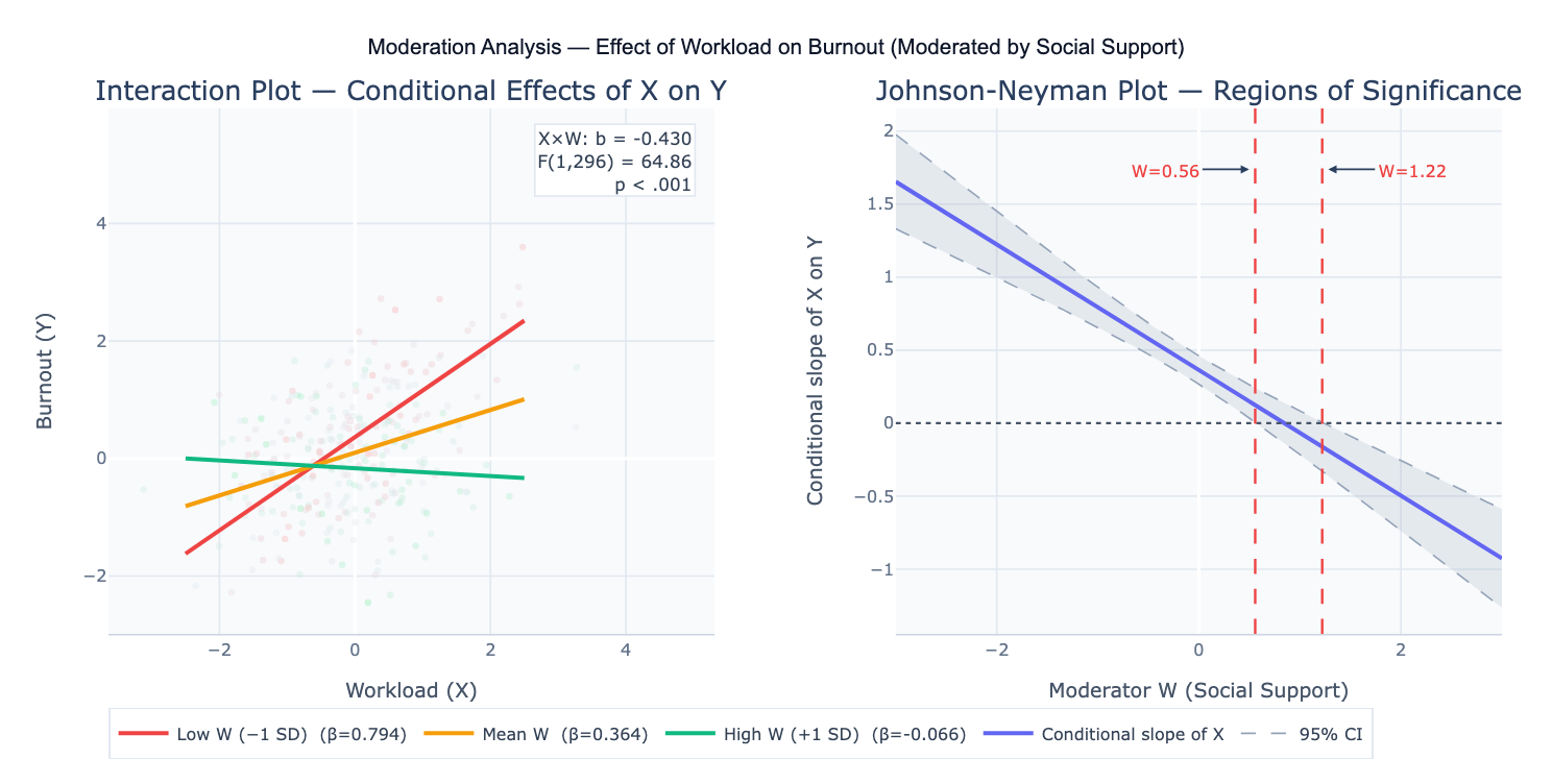
A concrete example: a workplace study measures workload (X), burnout (Y), and social support (W) in 300 employees. The interaction term b₃ = −0.43 (p < .001) indicates that high social support buffers the workload-burnout relationship — the interaction plot shows a steep positive slope between workload and burnout for employees with low support, a flat slope for those with average support, and a slightly negative slope for those with high support. The Johnson-Neyman technique identifies the exact value of W (social support score = 0.56) above which the effect of workload on burnout is no longer statistically significant — providing a precise threshold for the buffering effect.
How It Works
- Upload your data — provide a CSV or Excel file with one column each for the predictor (X), moderator (W), and outcome (Y), plus any covariates. All variables should be numeric and continuous (for a binary moderator, describe it as a dummy-coded 0/1 variable).
- Describe the analysis — e.g. "X = workload, W = social support, Y = burnout; mean-center X and W; test X×W interaction; interaction plot at low/mean/high W; Johnson-Neyman regions of significance; report all coefficients with 95% CI"
- Get full results — the AI writes Python code using statsmodels and Plotly to mean-center predictors, fit the interaction model, test the interaction term, plot conditional slopes, and produce the Johnson-Neyman significance region plot
Required Data Format
| Column | Description | Example |
|---|---|---|
X | Predictor variable | workload, dose, income |
W | Moderator variable | support, age, condition |
Y | Outcome variable | burnout, response, satisfaction |
covariate | Optional: control variables | gender, tenure, baseline |
Any column names work — describe them in your prompt. All variables should be numeric. For binary moderators (e.g., gender), code as 0/1 and interpret the interaction as the difference in X→Y slopes between groups. For categorical moderators with 3+ levels, dummy-code them and test a series of two-way interactions.
Interpreting the Results
| Output | What it means |
|---|---|
| b₁ (main effect of X) | Effect of X on Y when W = 0 (or W = mean, if centered) |
| b₂ (main effect of W) | Effect of W on Y when X = 0 (or X = mean, if centered) |
| b₃ (interaction X×W) | Change in the X→Y slope for each 1-unit increase in W — the key moderation coefficient |
| F-test for interaction | Significance test for b₃ — p < .05 indicates significant moderation |
| Conditional slope of X at W levels | b₁ + b₃×W — the X→Y slope at specific W values (−1 SD, mean, +1 SD) |
| Simple slope t-tests | Test whether the conditional slope is significantly different from zero at each W level |
| Johnson-Neyman region | Range of W values where the X→Y effect is statistically significant (p < .05) |
| Interaction plot | Visualization of X→Y regression lines at low, mean, and high W |
| ΔR² | Change in R² when adding the interaction term — effect size of the moderation |
Example Prompts
| Scenario | What to type |
|---|---|
| Basic moderation | X = stress, W = resilience, Y = wellbeing; mean-center X and W; test interaction; interaction plot; JN regions |
| Binary moderator | W is binary (0=female, 1=male); test if gender moderates X→Y; report conditional slopes for each group |
| Covariates | moderation controlling for age and baseline; include as covariates in the model; report adjusted interaction effect |
| Curvilinear moderation | test both linear and quadratic moderation: add X², W², and X²×W terms; compare model fit |
| ΔR² effect size | report ΔR² when adding interaction term; report f² (Cohen's f-squared) for the interaction |
| Pick-a-point probing | probe interaction at W = 10, 20, 30 (specific meaningful values); simple slope at each; t-test and CI |
| Moderated mediation | moderated mediation: X→M→Y with W moderating the a path (X→M); conditional indirect effects at 3 W levels |
| Three-way interaction | X × W × Z three-way interaction; test if Z moderates the X×W moderation; plot at 4 combinations of W and Z |
Assumptions to Check
- Linearity of main effects — moderation analysis assumes the main effects of X and W on Y are linear; inspect residual plots and scatterplots before adding the interaction; if either X or W has a non-linear relationship with Y, the interaction test may be confounded by the non-linearity
- Mean-centering — always center X and W (subtract their means) before computing the product term X×W; failing to center does not affect the interaction coefficient b₃ or its significance, but causes multicollinearity between main effects and the interaction term, inflating standard errors and making main effect coefficients uninterpretable
- Homoscedasticity — interaction models are particularly sensitive to heteroscedasticity; the variance of Y may increase with X×W; inspect residual plots and consider using heteroscedasticity-consistent (HC) standard errors (White correction) if variance is non-constant
- No extreme outliers — leverage points at the extremes of X×W can strongly influence the interaction estimate; identify observations with high leverage (hat values) and Cook's distance; consider robust regression if outliers are influential
- Sample size for interactions — detecting interaction effects requires substantially more power than detecting main effects; the interaction effect size (ΔR²) is typically much smaller than main effect R²; rule of thumb: n ≥ 200 for typical interaction effects (b₃ corresponding to ΔR² ≈ 0.01–0.02); simulation studies suggest many published moderation studies are severely underpowered
- Measurement reliability — unreliability in X or W attenuates the interaction coefficient (b₃) more than it attenuates main effects; if X or W are measured with error, the true interaction may be substantially larger than the observed b₃
Related Tools
Use the Mediation Analysis Calculator when X affects Y through M (mechanism question) rather than when W changes the X→Y relationship (context question) — mediation and moderation address different research questions, though they can be combined as moderated mediation. Use the Multiple Regression calculator to fit the regression model without the interaction term and compare R² — the ΔR² attributable to the interaction term is the effect size of the moderation. Use the Online two-way ANOVA calculator when both X and W are categorical — two-way ANOVA is a special case of moderation with categorical factors. Use the Partial Correlation Calculator to examine whether the X-Y correlation changes substantially when W is controlled — a large change suggests W may act as a moderator or mediator.
Frequently Asked Questions
What is the difference between moderation and mediation?Mediation asks "how?" or "through what mechanism?" — X affects M, which in turn affects Y; the mediator M is on the causal pathway from X to Y. Moderation asks "when?" or "for whom?" — W changes the strength or direction of the X→Y relationship; the moderator W is not on the X→Y causal path but interacts with X to affect Y. Example: stress (X) → burnout (Y) could be mediated by poor sleep (M: stress causes poor sleep, which causes burnout) or moderated by social support (W: the stress-burnout relationship is weaker when support is high). The two can be combined: moderated mediation tests whether the mediated path (X→M→Y) is stronger at some levels of W than others.
Why is the interaction term often non-significant even when I expect moderation? Moderation effects are typically small — interaction terms account for ΔR² ≈ 0.01–0.03 in most social science and health research, compared to main effects that may account for ΔR² > 0.10. This means interaction tests require large samples (n ≥ 200–500) to achieve adequate power. Additional reasons for low power: (1) measurement error in X or W attenuates the interaction coefficient substantially; (2) range restriction — if X or W have limited variance in your sample, the interaction cannot emerge; (3) non-linear moderation — if the true moderation is not linear (e.g., only extreme values of W moderate X→Y), the linear interaction term will miss it. Before concluding no moderation exists, consider whether your design and sample size had adequate power to detect the expected effect size.
What is the Johnson-Neyman technique and when should I use it? The Johnson-Neyman (J-N) technique finds the exact value(s) of the moderator W at which the conditional effect of X on Y transitions between statistically significant and non-significant. Instead of probing the interaction at arbitrary W levels (−1 SD, mean, +1 SD), J-N provides the precise boundary. For example, if the J-N boundary is at W = 12.4, the X→Y effect is significant for all W < 12.4 (assuming a negative interaction) but non-significant for W ≥ 12.4. Always check what proportion of your sample falls in each region — if 90% of participants are in the non-significant region, the significant effect at low W may be driven by a small fraction of observations. Use J-N alongside the interaction plot for complete interpretation.
Should I report b₃, simple slopes, or ΔR² as my primary effect size? Report all three: (1) b₃ with 95% CI and p-value (unstandardized) gives the raw interaction coefficient; standardized b₃ (when X, W, Y are all z-scored) allows comparison across studies; (2) ΔR² is the variance-explained effect size for the interaction — small ≈ 0.005, medium ≈ 0.01, large ≈ 0.025 (Frazier et al., 2004); (3) simple slopes at meaningful W levels give practical interpretation of the conditional effects. For meta-analyses, the standardized interaction coefficient is most useful. For applied reporting to non-statisticians, the interaction plot with labeled simple slopes is often most accessible.